برچسب: Dynamic

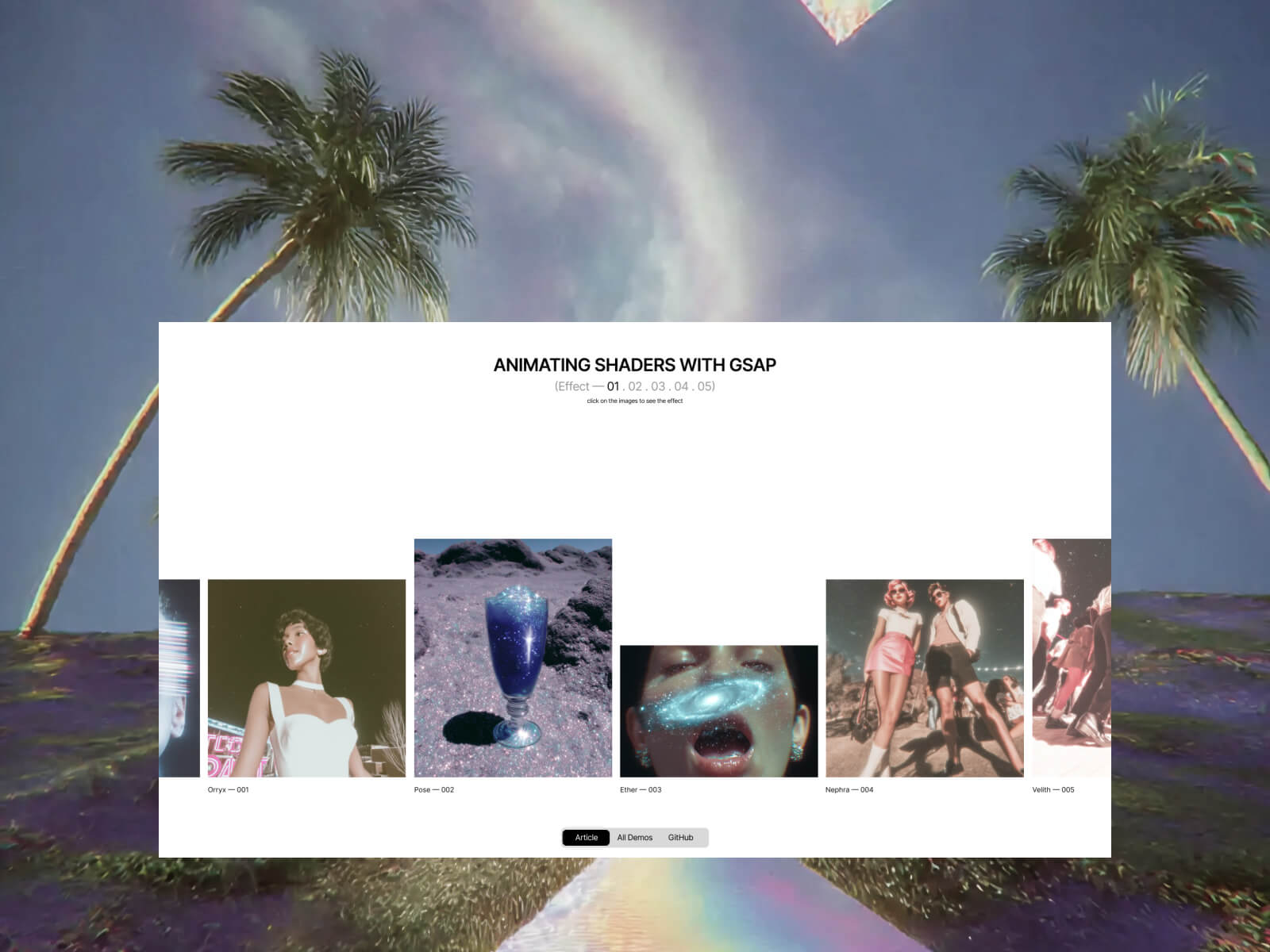
In this tutorial, we’ll explore how to bring motion and interactivity to your WebGL projects by combining GSAP with custom shaders. Working with the Dev team at Adoratorio Studio, I’ll guide you through four GPU-powered effects, from ripples that react to clicks to dynamic blurs that respond to scroll and drag.

We’ll start by setting up a simple WebGL scene and syncing it with our HTML layout. From there, we’ll move step by step through more advanced interactions, animating shader uniforms, blending textures, and revealing images through masks, until we turn everything into a scrollable, animated carousel.

By the end, you’ll understand how to connect GSAP timelines with shader parameters to create fluid, expressive visuals that react in real time and form the foundation for your own immersive web experiences.

Creating the HTML structure

As a first step, we will set up the page using HTML.

We will create a container without specifying its dimensions, allowing it to extend beyond the page width. Then, we will set the main container’s overflow property to hidden, as the page will be later made interactive through the GSAP Draggable and ScrollTrigger functionalities.

<main>
  <section class="content">
    <div class="content__carousel">
      <div class="content__carousel-inner-static">
        <div class="content__carousel-image">
          <img src="/images/01.webp" alt="" role="presentation">
          <span>Lorem — 001</span>
        </div>
        <div class="content__carousel-image">
          <img src="/images/04.webp" alt="" role="presentation">
          <span>Ipsum — 002</span>
        </div>
        <div class="content__carousel-image">
          <img src="/images/02.webp" alt="" role="presentation">
          <span>Dolor — 003</span>
        </div>
        ...
      </div>
    </div>
  </section>
</main>

We’ll style all this and then move on to the next step.

Sync between HTML and Canvas

We can now begin integrating Three.js into our project by creating a Stage class responsible for managing all 3D engine logic. Initially, this class will set up a renderer, a scene, and a camera.

We will pass an HTML node as the first parameter, which will act as the container for our canvas.
Next, we will update the CSS and the main script to create a full-screen canvas that resizes responsively and renders on every GSAP frame.

export default class Stage {
  constructor(container) {
    this.container = container;

    this.DOMElements = [...this.container.querySelectorAll('img')];

    this.renderer = new WebGLRenderer({
      powerPreference: 'high-performance',
      antialias: true,
      alpha: true,
    });
    this.renderer.setPixelRatio(Math.min(1.5, window.devicePixelRatio));
    this.renderer.setSize(window.innerWidth, window.innerHeight);
    this.renderer.domElement.classList.add('content__canvas');

    this.container.appendChild(this.renderer.domElement);

    this.scene = new Scene();

    const { innerWidth: width, innerHeight: height } = window;
    this.camera = new OrthographicCamera(-width / 2, width / 2, height / 2, -height / 2, -1000, 1000);
    this.camera.position.z = 10;
  }

  resize() {
    // Update camera props to fit the canvas size
    const { innerWidth: screenWidth, innerHeight: screenHeight } = window;

    this.camera.left = -screenWidth / 2;
    this.camera.right = screenWidth / 2;
    this.camera.top = screenHeight / 2;
    this.camera.bottom = -screenHeight / 2;
    this.camera.updateProjectionMatrix();

    // Update also planes sizes
    this.DOMElements.forEach((image, index) => {
      const { width: imageWidth, height: imageHeight } = image.getBoundingClientRect();
      this.scene.children[index].scale.set(imageWidth, imageHeight, 1);
    });

    // Update the render using the window sizes
    this.renderer.setSize(screenWidth, screenHeight);
  }

  render() {
    this.renderer.render(this.scene, this.camera);
  }
}

Back in our main.js file, we’ll first handle the stage’s resize event. After that, we’ll synchronize the renderer’s requestAnimationFrame (RAF) with GSAP by using gsap.ticker.add, passing the stage’s render function as the callback.

// Update resize with the stage resize
function resize() {
  ...
  stage.resize();
}

// Add render cycle to gsap ticker
gsap.ticker.add(stage.render.bind(stage));

<style>
.content__canvas {
  position: absolute;
  top: 0;
  left: 0;
  width: 100vw;
  height: 100svh;

  z-index: 2;
  pointer-events: none;
}
</style>

It’s now time to load all the images included in the HTML. For each image, we will create a plane and add it to the scene. To achieve this, we’ll update the class by adding two new methods:

setUpPlanes() {
  this.DOMElements.forEach((image) => {
    this.scene.add(this.generatePlane(image));
  });
}

generatePlane(image, ) {
  const loader = new TextureLoader();
  const texture = loader.load(image.src);

  texture.colorSpace = SRGBColorSpace;
  const plane = new Mesh(
    new PlaneGeometry(1, 1),
    new MeshStandardMaterial(),
  );

  return plane;
}

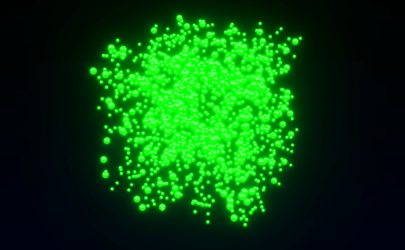
We can then call setUpPlanes() within the constructor of our Stage class.
The result should resemble the following, depending on the camera’s z-position or the planes’ placement—both of which can be adjusted to fit our specific needs.

The next step is to position the planes precisely to correspond with the location of their associated images and update their positions on each frame. To achieve this, we will implement a utility function that converts screen space (CSS pixels) into world space, leveraging the Orthographic Camera, which is already aligned with the screen.

const getWorldPositionFromDOM = (element, camera) => {
  const rect = element.getBoundingClientRect();

  const xNDC = (rect.left + rect.width / 2) / window.innerWidth * 2 - 1;
  const yNDC = -((rect.top + rect.height / 2) / window.innerHeight * 2 - 1);

  const xWorld = xNDC * (camera.right - camera.left) / 2;
  const yWorld = yNDC * (camera.top - camera.bottom) / 2;

  return new Vector3(xWorld, yWorld, 0);
};

render() {
  this.renderer.render(this.scene, this.camera);

  // For each plane and each image update the position of the plane to match the DOM element position on page
  this.DOMElements.forEach((image, index) => {
     this.scene.children[index].position.copy(getWorldPositionFromDOM(image, this.camera, this.renderer));
  });
}

By hiding the original DOM carousel, we can now display only the images as planes within the canvas. Create a simple class extending ShaderMaterial and use it in place of MeshStandardMaterial for the planes.

const plane = new Mesh(
  new PlaneGeometry(1, 1),
  new PlanesMaterial(),
);
...

import { ShaderMaterial } from 'three';
import baseVertex from './base.vert?raw';
import baseFragment from './base.frag?raw';

export default class PlanesMaterial extends ShaderMaterial {
  constructor() {
    super({
      vertexShader: baseVertex,
      fragmentShader: baseFragment,
    });
  }
}

// base.vert
varying vec2 vUv;

void main() {
  gl_Position = projectionMatrix * modelViewMatrix * vec4(position, 1.0);
  vUv = uv;
}

// base.frag
varying vec2 vUv;

void main() {
  gl_FragColor = vec4(vUv.x, vUv.y, 0.0, 1.0);
}

We can then replace the shader output with texture sampling based on the UV coordinates, passing the texture to the material and shaders as a uniform.

...
const plane = new Mesh(
  new PlaneGeometry(1, 1),
  new PlanesMaterial(texture),
);
...

export default class PlanesMaterial extends ShaderMaterial {
  constructor(texture) {
    super({
      vertexShader: baseVertex,
      fragmentShader: baseFragment,
      uniforms: {
        uTexture: { value: texture },
      },
    });
  }
}

// base.frag
varying vec2 vUv;

uniform sampler2D uTexture;

void main() {
  vec4 diffuse = texture2D(uTexture, vUv);
  gl_FragColor = diffuse;
}

Click on the images for a ripple and coloring effect

This steps breaks down the creation of an interactive grayscale transition effect, emphasizing the relationship between JavaScript (using GSAP) and GLSL shaders.

Step 1: Instant Color/Grayscale Toggle

Let’s start with the simplest version: clicking the image makes it instantly switch between color and grayscale.

The JavaScript (GSAP)

At this stage, GSAP’s role is to act as a simple “on/off” switch so let’s create a GSAP Observer to monitor the mouse click interaction:

this.observer = Observer.create({
  target: document.querySelector('.content__carousel'),
  type: 'touch,pointer',
  onClick: e => this.onClick(e),
});

And here come the following steps:

• Click Detection: We use an Observer to detect a click on our plane.
• State Management: A boolean flag, isBw (is Black and White), is toggled on each click.
• Shader Update: We use gsap.set() to instantly change a uniform in our shader. We’ll call it uGrayscaleProgress.
  • If isBw is true, uGrayscaleProgress becomes 1.0.
  • If isBw is false, uGrayscaleProgress becomes 0.0.

onClick(e) {
  if (intersection) {
    const { material, userData } = intersection.object;

    userData.isBw = !userData.isBw;

    gsap.set(material.uniforms.uGrayscaleProgress, {
      value: userData.isBw ? 1.0 : 0.0
    });
  }
}

The Shader (GLSL)

The fragment shader is very simple. It receives uGrayscaleProgress and uses it as a switch.

uniform sampler2D uTexture;
uniform float uGrayscaleProgress; // Our "switch" (0.0 or 1.0)
varying vec2 vUv;

vec3 toGrayscale(vec3 color) {
  float gray = dot(color, vec3(0.299, 0.587, 0.114));
  return vec3(gray);
}

void main() {
  vec3 originalColor = texture2D(uTexture, vUv).rgb;
  vec3 grayscaleColor = toGrayscale(originalColor);
  
   vec3 finalColor = mix(originalColor, grayscaleColor, uGrayscaleProgress);
   gl_FragColor = vec4(finalColor, 1.0);
}

Step 2: Animated Circular Reveal

An instant switch is boring. Let’s make the transition a smooth, circular reveal that expands from the center.

The JavaScript (GSAP)

GSAP’s role now changes from a switch to an animator.
Instead of gsap.set(), we use gsap.to() to animate uGrayscaleProgress from 0 to 1 (or 1 to 0) over a set duration. This sends a continuous stream of values (0.0, 0.01, 0.02, …) to the shader.

gsap.to(material.uniforms.uGrayscaleProgress, {
  value: userData.isBw ? 1 : 0,
  duration: 1.5,
  ease: 'power2.inOut'
});

The Shader (GLSL)

The shader now uses the animated uGrayscaleProgress to define the radius of a circle.

void main() {
  float dist = distance(vUv, vec2(0.5));
  
  // 2. Create a circular mask.
  float mask = smoothstep(uGrayscaleProgress - 0.1, uGrayscaleProgress, dist);

  // 3. Mix the colors based on the mask's value for each pixel.
  vec3 finalColor = mix(originalColor, grayscaleColor, mask);
  gl_FragColor = vec4(finalColor, 1.0);
}

How smoothstep works here: Pixels where dist is less than uGrayscaleProgress – 0.1 get a mask value of 0. Pixels where dist is greater than uGrayscaleProgress get a value of 1. In between, it’s a smooth transition, creating the soft edge.

Step 3: Originating from the Mouse Click

The effect is much more engaging if it starts from the exact point of the click.

The JavaScript (GSAP)

We need to tell the shader where the click happened.

• Raycasting: We use a Raycaster to find the precise (u, v) texture coordinate of the click on the mesh.
• uMouse Uniform: We add a uniform vec2 uMouse to our material.
• GSAP Timeline: Before the animation starts, we use .set() on our GSAP timeline to update the uMouse uniform with the intersection.uv coordinates.

if (intersection) {
  const { material, userData } = intersection.object;

  material.uniforms.uMouse.value = intersection.uv;

  gsap.to(material.uniforms.uGrayscaleProgress, {
      value: userData.isBw ? 1 : 0
  });
}

The Shader (GLSL)

We simply replace the hardcoded center with our new uMouse uniform.

...
uniform vec2 uMouse; // The (u,v) coordinates from the click
...

void main() {
...

// 1. Calculate distance from the MOUSE CLICK, not the center.
float dist = distance(vUv, uMouse);
}

Important Detail: To ensure the circular reveal always covers the entire plane, even when clicking in a corner, we calculate the maximum possible distance from the click point to any of the four corners (getMaxDistFromCorners) and normalize our dist value with it: dist / maxDist.

This guarantees the animation completes fully.

Step 4: Adding the Final Ripple Effect

The last step is to add the 3D ripple effect that deforms the plane. This requires modifying the vertex shader.

The JavaScript (GSAP)

We need one more animated uniform to control the ripple’s lifecycle.

1. uRippleProgress Uniform: We add a uniform float uRippleProgress.
2. GSAP Keyframes: In the same timeline, we animate uRippleProgress from 0 to 1 and back to 0. This makes the wave rise up and then settle back down.

gsap.timeline({ defaults: { duration: 1.5, ease: 'power3.inOut' } })
  .set(material.uniforms.uMouse, { value: intersection.uv }, 0)
  .to(material.uniforms.uGrayscaleProgress, { value: 1 }, 0)
  .to(material.uniforms.uRippleProgress, {
      keyframes: { value: [0, 1, 0] } // Rise and fall
  }, 0)

The Shaders (GLSL)

High-Poly Geometry: To see a smooth deformation, the PlaneGeometry in Three.js must be created with many segments (e.g., new PlaneGeometry(1, 1, 50, 50)). This gives the vertex shader more points to manipulate.

generatePlane(image, ) {
  ...
  const plane = new Mesh(
    new PlaneGeometry(1, 1, 50, 50),
    new PlanesMaterial(texture),
  );

  return plane;
}

Vertex Shader: This shader now calculates the wave and moves the vertices.

uniform float uRippleProgress;
uniform vec2 uMouse;
varying float vRipple; // Pass the ripple intensity to the fragment shader

void main() {
  vec3 pos = position;
  float dist = distance(uv, uMouse);

  float ripple = sin(-PI * 10.0 * (dist - uTime * 0.1));
  ripple *= uRippleProgress;

  pos.y += ripple * 0.1;

  vRipple = ripple;
  gl_Position = projectionMatrix * modelViewMatrix * vec4(pos, 1.0);
}

Fragment Shader: We can use the ripple intensity to add a final touch, like making the wave crests brighter.

varying float vRipple; // Received from vertex shader

void main() {
  // ... (all the color and mask logic from before)
  vec3 color = mix(color1, color2, mask);

  // Add a highlight based on the wave's height
  color += vRipple * 2.0;

  gl_FragColor = vec4(color, diffuse.a);
}

By layering these techniques, we create a rich, interactive effect where JavaScript and GSAP act as the puppet master, telling the shaders what to do, while the shaders handle the heavy lifting of drawing it beautifully and efficiently on the GPU.

Step 5: Reverse effect on previous tile

As a final step, we set up a reverse animation of the current tile when a new tile is clicked. Let’s start by creating the reset animation that reverses the animation of the uniforms:

resetMaterial(object) {
  // Reset all shader uniforms to default values
  gsap.timeline({
    defaults: { duration: 1, ease: 'power2.out' },

    onUpdate() {
      object.material.uniforms.uTime.value += 0.1;
    },
    onComplete() {       
      object.userData.isBw = false;
    }
  })
  .set(object.material.uniforms.uMouse, { value: { x: 0.5, y: 0.5} }, 0)
  .set(object.material.uniforms.uDirection, { value: 1.0 }, 0)
  .fromTo(object.material.uniforms.uGrayscaleProgress, { value: 1 }, { value: 0 }, 0)
  .to(object.material.uniforms.uRippleProgress, { keyframes: { value: [0, 1, 0] } }, 0);
}

Now, at each click, we need to set the current tile so that it’s saved in the constructor, allowing us to pass the current material to the reset animation. Let’s modify the onClick function like this and analyze it step by step:

if (this.activeObject && intersection.object !== this.activeObject && this.activeObject.userData.isBw) {
  this.resetMaterial(this.activeObject)
  
  // Stops timeline if active
  if (this.activeObject.userData.tl?.isActive()) this.activeObject.userData.tl.kill();
  
  // Cleans timeline
  this.activeObject.userData.tl = null;
}

// Setup active object
this.activeObject = intersection.object;

• If this.activeObject exists (initially set to null in the constructor), we proceed to reset it to its initial black and white state
• If there’s a current animation on the active tile, we use GSAP’s kill method to avoid conflicts and overlapping animations
• We reset userData.tl to null (it will be assigned a new timeline value if the tile is clicked again)
• We then set the value of this.activeObject to the object selected via the Raycaster

In this way, we’ll have a double ripple animation: one on the clicked tile, which will be colored, and one on the previously active tile, which will be reset to its original black and white state.

Texture reveal mask effect

In this tutorial, we will create an interactive effect that blends two images on a plane when the user hovers or touches it.

Step 1: Setting Up the Planes

Unlike the previous examples, in this case we need different uniforms for the planes, as we are going to create a mix between a visible front texture and another texture that will be revealed through a mask that “cuts through” the first texture.

Let’s start by modifying the index.html file, adding a data attribute to all images where we’ll specify the underlying texture:

<img src="/images/front-texture.webp" alt="" role="presentation" data-back="/images/back-texture.webp">

Then, inside our Stage.js, we’ll modify the generatePlane method, which is used to create the planes in WebGL. We’ll start by retrieving the second texture to load via the data attribute, and we’ll pass the plane material the parameters with both textures and the aspect ratio of the images:

generatePlane(image) {
  const loader = new TextureLoader();
  const texture = loader.load(image.src);
  const textureBack = loader.load(image.dataset.back);

  texture.colorSpace = SRGBColorSpace;
  textureBack.colorSpace = SRGBColorSpace;

  const { width, height } = image.getBoundingClientRect();

  const plane = new Mesh(
    new PlaneGeometry(1, 1),
    new PlanesMaterial(texture, textureBack, height / width),
  );

  return plane;
}

Step 2: Material Setup

import { ShaderMaterial, Vector2 } from 'three';
import baseVertex from './base.vert?raw';
import baseFragment from './base.frag?raw';

export default class PlanesMaterial extends ShaderMaterial {
  constructor(texture, textureBack, imageRatio) {
    super({
      vertexShader: baseVertex,
      fragmentShader: baseFragment,
      uniforms: {
        uTexture: { value: texture },
        uTextureBack: { value: textureBack },
        uMixFactor: { value: 0.0 },
        uAspect: { value: imageRatio },
        uMouse: { value: new Vector2(0.5, 0.5) },
      },
    });
  }
}

Let’s quickly analyze the uniforms passed to the material:

• uTexture and uTextureBack are the two textures shown on the front and through the mask
• uMixFactor represents the blending value between the two textures inside the mask
• uAspect is the aspect ratio of the images used to calculate a circular mask
• uMouse represents the mouse coordinates, updated to move the mask within the plane

Step 3: The Javascript (GSAP)

this.observer = Observer.create({
  target: document.querySelector('.content__carousel'),
  type: 'touch,pointer',
  onMove: e => this.onMove(e),
  onHoverEnd: () => this.hoverOut(),
});

Quickly, let’s create a GSAP Observer to monitor the mouse movement, passing two functions:

• onMove checks, using the Raycaster, whether a plane is being hit in order to manage the opening of the reveal mask
• onHoverEnd is triggered when the cursor leaves the target area, so we’ll use this method to reset the reveal mask’s expansion uniform value back to 0.0

Let’s go into more detail on the onMove function to explain how it works:

onMove(e) {
  const normCoords = {
    x: (e.x / window.innerWidth) * 2 - 1,
    y: -(e.y / window.innerHeight) * 2 + 1,
  };

  this.raycaster.setFromCamera(normCoords, this.camera);

  const [intersection] = this.raycaster.intersectObjects(this.scene.children);

  if (intersection) {
    this.intersected = intersection.object;
    const { material } = intersection.object;

    gsap.timeline()
      .set(material.uniforms.uMouse, { value: intersection.uv }, 0)
      .to(material.uniforms.uMixFactor, { value: 1.0, duration: 3, ease: 'power3.out' }, 0);
  } else {
    this.hoverOut();
  }
}

In the onMove method, the first step is to normalize the mouse coordinates from -1 to 1 to allow the Raycaster to work with the correct coordinates.

On each frame, the Raycaster is then updated to check if any object in the scene is intersected. If there is an intersection, the code saves the hit object in a variable.

When an intersection occurs, we proceed to work on the animation of the shader uniforms.

Specifically, we use GSAP’s set method to update the mouse position in uMouse, and then animate the uMixFactor variable from 0.0 to 1.0 to open the reveal mask and show the underlying texture.

If the Raycaster doesn’t find any object under the pointer, the hoverOut method is called.

hoverOut() {
    if (!this.intersected) return;

    // Stop any running tweens on the uMixFactor uniform
    gsap.killTweensOf(this.intersected.material.uniforms.uMixFactor);

    // Animate uMixFactor back to 0 smoothly
    gsap.to(this.intersected.material.uniforms.uMixFactor, { value: 0.0, duration: 0.5, ease: 'power3.out });

    // Clear the intersected reference
    this.intersected = null;
  }

This method handles closing the reveal mask once the cursor leaves the plane.

First, we rely on the killAllTweensOf method to prevent conflicts or overlaps between the mask’s opening and closing animations by stopping all ongoing animations on the uMixFactor .

Then, we animate the mask’s closing by setting the uMixFactor uniform back to 0.0 and reset the variable that was tracking the currently highlighted object.

Step 4: The Shader (GLSL)

uniform sampler2D uTexture;
uniform sampler2D uTextureBack;
uniform float uMixFactor;
uniform vec2 uMouse;
uniform float uAspect;

varying vec2 vUv;

void main() {
    vec2 correctedUv = vec2(vUv.x, (vUv.y - 0.5) * uAspect + 0.5);
    vec2 correctedMouse = vec2(uMouse.x, (uMouse.y - 0.5) * uAspect + 0.5);
    
    float distance = length(correctedUv - correctedMouse);
    float influence = 1.0 - smoothstep(0.0, 0.5, distance);

    float finalMix = uMixFactor * influence;

    vec4 textureFront = texture2D(uTexture, vUv);
    vec4 textureBack = texture2D(uTextureBack, vUv);

    vec4 finalColor = mix(textureFront, textureBack, finalMix);

    gl_FragColor = finalColor;
}

Inside the main() function, it starts by normalizing the UV coordinates and the mouse position relative to the image’s aspect ratio. This correction is applied because we are using non-square images, so the vertical coordinates must be adjusted to keep the mask’s proportions correct and ensure it remains circular. Therefore, the vUv.y and uMouse.y coordinates are modified so they are “scaled” vertically according to the aspect ratio.

At this point, the distance is calculated between the current pixel (correctedUv) and the mouse position (correctedMouse). This distance is a numeric value that indicates how close or far the pixel is from the mouse center on the surface.

We then move on to the actual creation of the mask. The uniform influence must vary from 1 at the cursor’s center to 0 as it moves away from the center. We use the smoothstep function to recreate this effect and obtain a soft, gradual transition between two values, so the effect naturally fades.

The final value for the mix between the two textures, that is the finalMix uniform, is given by the product of the global factor uMixFactor (which is a static numeric value passed to the shader) and this local influence value. So the closer a pixel is to the mouse position, the more its color will be influenced by the second texture, uTextureBack.

The last part is the actual blending: the two colors are mixed using the mix() function, which creates a linear interpolation between the two textures based on the value of finalMix. When finalMix is 0, only the front texture is visible.

When it is 1, only the background texture is visible. Intermediate values create a gradual blend between the two textures.

Click & Hold mask reveal effect

This document breaks down the creation of an interactive effect that transitions an image from color to grayscale. The effect starts from the user’s click, expanding outwards with a ripple distortion.

Step 1: The “Move” (Hover) Effect

In this step, we’ll create an effect where an image transitions to another as the user hovers their mouse over it. The transition will originate from the pointer’s position and expand outwards.

The JavaScript (GSAP Observer for onMove)

GSAP’s Observer plugin is the perfect tool for tracking pointer movements without the boilerplate of traditional event listeners.

• Setup Observer: We create an Observer instance that targets our main container and listens for touch and pointer events. We only need the onMove and onHoverEnd callbacks.
• onMove(e) Logic:
  When the pointer moves, we use a Raycaster to determine if it’s over one of our interactive images.
  • If an object is intersected, we store it in this.intersected.
  • We then use a GSAP Timeline to animate the shader’s uniforms.
  • uMouse: We instantly set this vec2 uniform to the pointer’s UV coordinate on the image. This tells the shader where the effect should originate.
  • uMixFactor: We animate this float uniform from 0 to 1. This uniform will control the blend between the two textures in the shader.
• onHoverEnd() Logic:
  • When the pointer leaves the object, Observer calls this function.
  • We kill any ongoing animations on uMixFactor to prevent conflicts.
  • We animate uMixFactor back to 0, reversing the effect.

Code Example: the “Move” effect

This code shows how Observer is configured to handle the hover interaction.

import { gsap } from 'gsap';
import { Observer } from 'gsap/Observer';
import { Raycaster } from 'three';

gsap.registerPlugin(Observer);

export default class Effect {
  constructor(scene, camera) {
    this.scene = scene;
    this.camera = camera;
    this.intersected = null;
    this.raycaster = new Raycaster();

	// 1. Create the Observer
	this.observer = Observer.create({
      target: document.querySelector('.content__carousel'),
      type: 'touch,pointer',
      onMove: e => this.onMove(e),
      onHoverEnd: () => this.hoverOut(), // Called when the pointer leaves the target
    });
  }

  hoverOut() {
    if (!this.intersected) return;

	// 3. Animate the effect out
    gsap.killTweensOf(this.intersected.material.uniforms.uMixFactor);
    gsap.to(this.intersected.material.uniforms.uMixFactor, {
      value: 0.0,
      duration: 0.5,
      ease: 'power3.out'
    });

    this.intersected = null;
  }

  onMove(e) {
	// ... (Raycaster logic to find intersection)
	const [intersection] = this.raycaster.intersectObjects(this.scene.children);

    if (intersection) {
      this.intersected = intersection.object;
      const { material } = intersection.object;

	  // 2. Animate the uniforms on hover
      gsap.timeline()
        .set(material.uniforms.uMouse, { value: intersection.uv }, 0) // Set origin point
        .to(material.uniforms.uMixFactor, { // Animate the blendvalue: 1.0,
          duration: 3,
          ease: 'power3.out'
        }, 0);
    } else {
      this.hoverOut(); // Reset if not hovering over anything
    }
  }
}

The Shader (GLSL)

The fragment shader receives the uniforms animated by GSAP and uses them to draw the effect.

• uMouse: Used to calculate the distance of each pixel from the pointer.
• uMixFactor: Used as the interpolation value in a mix() function. As it animates from 0 to 1, the shader smoothly blends from textureFront to textureBack.
• smoothstep(): We use this function to create a circular mask that expands from the uMouse position. The radius of this circle is controlled by uMixFactor.

uniform sampler2D uTexture; // Front image
uniform sampler2D uTextureBack; // Back image
uniform float uMixFactor; // Animated by GSAP (0 to 1)
uniform vec2 uMouse; // Set by GSAP on move

// ...

void main() {
  // ... (code to correct for aspect ratio)

  // 1. Calculate distance of the current pixel from the mouse
  float distance = length(correctedUv - correctedMouse);

  // 2. Create a circular mask that expands as uMixFactor increases
  float influence = 1.0 - smoothstep(0.0, 0.5, distance);
  float finalMix = uMixFactor * influence;

  // 3. Read colors from both textures
  vec4 textureFront = texture2D(uTexture, vUv);
  vec4 textureBack = texture2D(uTextureBack, vUv);

  // 4. Mix the two textures based on the animated value
  vec4 finalColor = mix(textureFront, textureBack, finalMix);
	
  gl_FragColor = finalColor;
}

Step 2: The “Click & Hold” Effect

Now, let’s build a more engaging interaction. The effect will start when the user presses down, “charge up” while they hold, and either complete or reverse when they release.

The JavaScript (GSAP)

Observer makes this complex interaction straightforward by providing clear callbacks for each state.

• Setup Observer: This time, we configure Observer to use onPress, onMove, and onRelease.
• onPress(e):
  • When the user presses down, we find the intersected object and store it in this.active.
  • We then call onActiveEnter(), which starts a GSAP timeline for the “charging” animation.
• onActiveEnter():
  • This function defines the multi-stage animation. We use await with a GSAP tween to create a sequence.
  • First, it animates uGrayscaleProgress to a midpoint (e.g., 0.35) and holds it. This is the “hold” part of the interaction.
  • If the user continues to hold, a second tween completes the animation, transitioning uGrayscaleProgress to 1.0.
  • An onComplete callback then resets the state, preparing for the next interaction.
• onRelease():
  • If the user releases the pointer before the animation completes, this function is called.
  • It calls onActiveLeve(), which kills the “charging” animation and animates uGrayscaleProgress back to 0, effectively reversing the effect.
• onMove(e):
  • This is still used to continuously update the uMouse uniform, so the shader’s noise effect tracks the pointer even during the hold.
  • Crucially, if the pointer moves off the object, we call onRelease() to cancel the interaction.

Code Example: Click & Hold

This code demonstrates the press, hold, and release logic managed by Observer.

import { gsap } from 'gsap';
import { Observer } from 'gsap/Observer';

// ...

export default class Effect {
  constructor(scene, camera) {
	// ...
		
    this.active = null; // Currently active (pressed) object
	this.raycaster = new Raycaster();
	
	// 1. Create the Observer for press, move, and release
	this.observer = Observer.create({
	  target: document.querySelector('.content__carousel'),
	  type: 'touch,pointer',
      onPress: e => this.onPress(e),
      onMove: e => this.onMove(e),
	  onRelease: () => this.onRelease(),
	});
	
	// Continuously update uTime for the procedural effect
	gsap.ticker.add(() => {
	  if (this.active) {
	    this.active.material.uniforms.uTime.value += 0.1;
	  }
	});
  }

  // 3. The "charging" animation
  async onActiveEnter() {
    gsap.killTweensOf(this.active.material.uniforms.uGrayscaleProgress);

    // First part of the animation (the "hold" phase)
	await gsap.to(this.active.material.uniforms.uGrayscaleProgress, {
      value: 0.35,
      duration: 0.5,
    });

	// Second part, completes after the hold
    gsap.to(this.active.material.uniforms.uGrayscaleProgress, {
      value: 1,
      duration: 0.5,
      delay: 0.12,
      ease: 'power2.in',
      onComplete: () => {/* ... reset state ... */ },
    });
  }

  // 4. Reverses the animation on early release
  onActiveLeve(mesh) {
    gsap.killTweensOf(mesh.material.uniforms.uGrayscaleProgress);
    gsap.to(mesh.material.uniforms.uGrayscaleProgress, {
      value: 0,
      onUpdate: () => {
        mesh.material.uniforms.uTime.value += 0.1;
      },
    });
  }

  // ... (getIntersection logic) ...
	
  // 2. Handle the initial press
  onPress(e) {
    const intersection = this.getIntersection(e);

    if (intersection) {
      this.active = intersection.object;
      this.onActiveEnter(this.active); // Start the animation
    }
  }

  onRelease() {
    if (this.active) {
      const prevActive = this.active;
      this.active = null;
      this.onActiveLeve(prevActive); // Reverse the animation
    }
  }

  onMove(e) {
	// ... (getIntersection logic) ...
		
	if (intersection) {
	  // 5. Keep uMouse updated while holding
	  const { material } = intersection.object;
      gsap.set(material.uniforms.uMouse, { value: intersection.uv });
    } else {
      this.onRelease(); // Cancel if pointer leaves
    }
  }
}

The Shader (GLSL)

The fragment shader for this effect is more complex. It uses the animated uniforms to create a distorted, noisy reveal.

• uGrayscaleProgress: This is the main driver, animated by GSAP. It controls both the radius of the circular mask and the strength of a “liquid” distortion effect.
• uTime: This is continuously updated by gsap.ticker as long as the user is pressing. It’s used to add movement to the noise, making the effect feel alive and dynamic.
• noise() function: A standard GLSL noise function generates procedural, organic patterns. We use this to distort both the shape of the circular mask and the image texture coordinates (UVs).

// ... (uniforms and helper functions)

void main() {
  // 1. Generate a noise value that changes over time
  float noisy = (noise(vUv * 25.0 + uTime * 0.5) - 0.5) * 0.05;

  // 2. Create a distortion that pulses using the main progress animation
  float distortionStrength = sin(uGrayscaleProgress * PI) * 0.5;
  vec2 distortedUv = vUv + vec2(noisy) * distortionStrength;

  // 3. Read the texture using the distorted coordinates for a liquid effect
  vec4 diffuse = texture2D(uTexture, distortedUv);
  // ... (grayscale logic)
	
  // 4. Calculate distance from the mouse, but add noise to it
  float dist = distance(vUv, uMouse);
  float distortedDist = dist + noisy;

  // 5. Create the circular mask using the distorted distance and progress
  float maxDist = getMaxDistFromCorners(uMouse);
  float mask = smoothstep(uGrayscaleProgress - 0.1, uGrayscaleProgress, distortedDist / maxDist);

  // 6. Mix between the original and grayscale colors
  vec3 color = mix(color1, color2, mask);

  gl_FragColor = vec4(color, diffuse.a);
}

This shader combines noise-based distortion, smooth circular masking, and real-time uniform updates to create a liquid, organic transition that radiates from the click position. As GSAP animates the shader’s progress and time values, the effect feels alive and tactile — a perfect example of how animation logic in JavaScript can drive complex visual behavior directly on the GPU.

Dynamic blur effect carousel

Step 1: Create the carousel

In this final demo, we will create an additional implementation, turning the image grid into a scrollable carousel that can be navigated both by dragging and scrolling.

First we will implement the Draggable plugin by registering it and targeting the appropriate <div>
with the desired configuration. Make sure to handle boundary constraints and update them accordingly when the window is resized.

const carouselInnerRef = document.querySelector('.content__carousel-inner');
const draggable = new Draggable(carouselInnerRef, {
  type: 'x',
  inertia: true,
  dragResistance: 0.5,
  edgeResistance: 0.5,
  throwResistance: 0.5,
  throwProps: true,
});

function resize() {
  const innerWidth = carouselInnerRef.scrollWidth;
  const viewportWidth = window.innerWidth;
  maxScroll = Math.abs(Math.min(0, viewportWidth - innerWidth));

  draggable.applyBounds({ minX: -maxScroll, maxX: 0 });
}

window.addEventListener('resize', debounce(resize));

We ill also link GSAP Draggable to the scroll functionality using the GSAP ScrollTrigger plugin, allowing us to synchronize both scroll and drag behavior within the same container. Let’s explore this in more detail:

let maxScroll = Math.abs(Math.min(0, window.innerWidth - carouselInnerRef.scrollWidth));

const scrollTriggerInstance = ScrollTrigger.create({
  trigger: carouselWrapper,
  start: 'top top',
  end: `+=${2.5 * maxScroll}`,
  pin: true,
  scrub: 0.05,
  anticipatePin: 1,
  invalidateOnRefresh: true,
});

...

resize() {
  ...
  scrollTriggerInstance.refresh();
}

Now that ScrollTrigger is configured on the same container, we can focus on synchronizing the scroll position between both plugins, starting from the ScrollTrigger instance:

onUpdate(e) {
  const x = -maxScroll * e.progress;

  gsap.set(carouselInnerRef, { x });
  draggable.x = x;
  draggable.update();
}

We then move on to the Draggable instance, which will be updated within both its onDrag and onThrowUpdate callbacks using the scrollPos variable. This variable will serve as the final scroll position for both the window and the ScrollTrigger instance.

onDragStart() {},
onDrag() {
  const progress = gsap.utils.normalize(draggable.maxX, draggable.minX, draggable.x);
  scrollPos = scrollTriggerInstance.start + (scrollTriggerInstance.end - scrollTriggerInstance.start) * progress;
  window.scrollTo({ top: scrollPos, behavior: 'instant' });

  scrollTriggerInstance.scroll(scrollPos);
},
onThrowUpdate() {
  const progress = gsap.utils.normalize(draggable.maxX, draggable.minX, draggable.x);
  scrollPos = scrollTriggerInstance.start + (scrollTriggerInstance.end - scrollTriggerInstance.start) * progress;
  window.scrollTo({ top: scrollPos, behavior: 'instant' });
},
onThrowComplete() {
  scrollTriggerInstance.scroll(scrollPos);
}

Step 2: Material setup

export default class PlanesMaterial extends ShaderMaterial {
  constructor(texture) {
    super({
      vertexShader: baseVertex,
      fragmentShader: baseFragment,
      uniforms: {
        uTexture: { value: texture },
        uBlurAmount: { value: 0 },
      },
    });
  }
}

Let’s quickly analyze the uniforms passed to the material:

• uTexture is the base texture rendered on the plane
• uBlurAmount represents the blur strength based on the distance from the window center

Step 3: The JavaScript (GSAP)

constructor(scene, camera) {
  ...
  this.callback = this.scrollUpdateCallback;
  this.centerX = window.innerWidth / 2
  ...
}

In the constructor we set up two pieces we’ll use to drive the dynamic blur effect:

• <strong>this.callback</strong> references the function used inside ScrollTrigger’s onUpdate to refresh the blur amount
• this.centerX represents the window center on X axes and is updated on each window resize

Let’s dive into the callback passed to ScrollTrigger:

scrollUpdateCallback() {
  this.tiles.forEach(tile => {
    const worldPosition = tile.getWorldPosition(new Vector3());
    const vector = worldPosition.clone().project(this.camera);

    const screenX = (vector.x * 0.5 + 0.5) * window.innerWidth;

    const distance = Math.abs(screenX - this.centerX);
    const maxDistance = window.innerWidth / 2;

    const blurAmount = MathUtils.clamp(distance / maxDistance * 5, 0.0, 5.0);

    gsap.to(tile.material.uniforms.uBlurAmount, {
      value: Math.round(blurAmount / 2) * 2,
      duration: 1.5,
      ease: 'power3.out'
    });
  });
}

Let’s dive deeper into this:

• Vector projects each plane’s 3D position into normalized device coordinates; .project(this.camera) converts to the -1..1 range, then it’s scaled to real screen pixel coordinates.
• screenX are the 2D screen-space coordinates.
• distance measures how far the plane is from the screen center.
• maxDistance is the maximum possible distance from center to corner.
• blurAmount computes blur strength based on distance from the center; it’s clamped between 0.0 and 5.0 to avoid extreme values that would harm visual quality or shader performance.
• The <strong>uBlurAmount</strong> uniform is animated toward the computed blurAmount. Rounding to the nearest even number (Math.round(blurAmount / 2) * 2) helps avoid overly frequent tiny changes that could cause visually unstable blur.

Step 4: The Shader (GLSL)

uniform sampler2D uTexture;
uniform float uBlurAmount;

varying vec2 vUv;

vec4 kawaseBlur(sampler2D tex, vec2 uv, float offset) {
  vec2 texelSize = vec2(1.0) / vec2(textureSize(tex, 0));
  
  vec4 color = vec4(0.0);
  
  color += texture2D(tex, uv + vec2(offset, offset) * texelSize);
  color += texture2D(tex, uv + vec2(-offset, offset) * texelSize);
  color += texture2D(tex, uv + vec2(offset, -offset) * texelSize);
  color += texture2D(tex, uv + vec2(-offset, -offset) * texelSize);
  
  return color * 0.25;
}

vec4 multiPassKawaseBlur(sampler2D tex, vec2 uv, float blurStrength) {
  vec4 baseTexture = texture2D(tex, uv);
  
  vec4 blur1 = kawaseBlur(tex, uv, 1.0 + blurStrength * 1.5);
  vec4 blur2 = kawaseBlur(tex, uv, 2.0 + blurStrength);
  vec4 blur3 = kawaseBlur(tex, uv, 3.0 + blurStrength * 2.5);
  
  float t1 = smoothstep(0.0, 3.0, blurStrength);
  float t2 = smoothstep(3.0, 7.0, blurStrength);
  
  vec4 blurredTexture = mix(blur1, blur2, t1);
  blurredTexture = mix(blurredTexture, blur3, t2);
  
  float mixFactor = smoothstep(0.0, 1.0, blurStrength);
  
  return mix(baseTexture, blurredTexture, mixFactor);
}

void main() {
  vec4 color = multiPassKawaseBlur(uTexture, vUv, uBlurAmount);
  gl_FragColor = color;
}

This GLSL fragment receives a texture (uTexture) and a dynamic value (uBlurAmount) indicating how much the plane should be blurred. Based on this value, the shader applies a multi-pass Kawase blur, an efficient technique that simulates a soft, pleasing blur while staying performant.

Let’s examine the kawaseBlur function, which applies a light blur by sampling 4 points around the current pixel (uv), each offset positively or negatively.

• texelSize computes the size of one pixel in UV coordinates so offsets refer to “pixel amounts” regardless of texture resolution.
• Four samples are taken in a diagonal cross pattern around uv.
• The four colors are averaged (multiplied by 0.25) to return a balanced result.

This function is a light single pass. To achieve a stronger effect, we apply it multiple times.

The multiPassKawaseBlur function does exactly that, progressively increasing blur and then blending the passes:

vec4 blur1 = kawaseBlur(tex, uv, 1.0 + blurStrength * 1.5);
vec4 blur2 = kawaseBlur(tex, uv, 2.0 + blurStrength);
vec4 blur3 = kawaseBlur(tex, uv, 3.0 + blurStrength * 2.5);

This produces a progressive, visually smooth result.

Next, we blend the different blur levels using two separate smoothsteps:

float t1 = smoothstep(0.0, 3.0, blurStrength);
float t2 = smoothstep(3.0, 7.0, blurStrength);
  
vec4 finalBlur = mix(blur1, blur2, t1);
finalBlur = mix(finalBlur, blur3, t2);

The first mix blends blur1 and blur2, while the second blends that result with blur3. The resulting finalBlur represents the Kawase-blurred texture, which we finally mix with the base texture passed via the uniform.

Finally, we mix the blurred texture with the original texture based on blurStrength, using another smoothstep from 0 to 1:

float mixFactor = smoothstep(0.0, 1.0, blurStrength);
return mix(baseTexture, finalBlur, mixFactor);

Final Words

Bringing together GSAP’s animation power and the creative freedom of GLSL shaders opens up a whole new layer of interactivity for the web. By animating shader uniforms directly with GSAP, we’re able to blend smooth motion design principles with the raw flexibility of GPU rendering — crafting experiences that feel alive, fluid, and tactile.

From simple grayscale transitions to ripple-based deformations and dynamic blur effects, every step in this tutorial demonstrates how motion and graphics can respond naturally to user input, creating interfaces that invite exploration rather than just observation.

While these techniques push the boundaries of front-end development, they also highlight a growing trend: the convergence of design, code, and real-time rendering.

So, take these examples, remix them, and make them your own — because the most exciting part of working with GSAP and shaders is that the canvas is quite literally infinite.