برچسب: Interactive

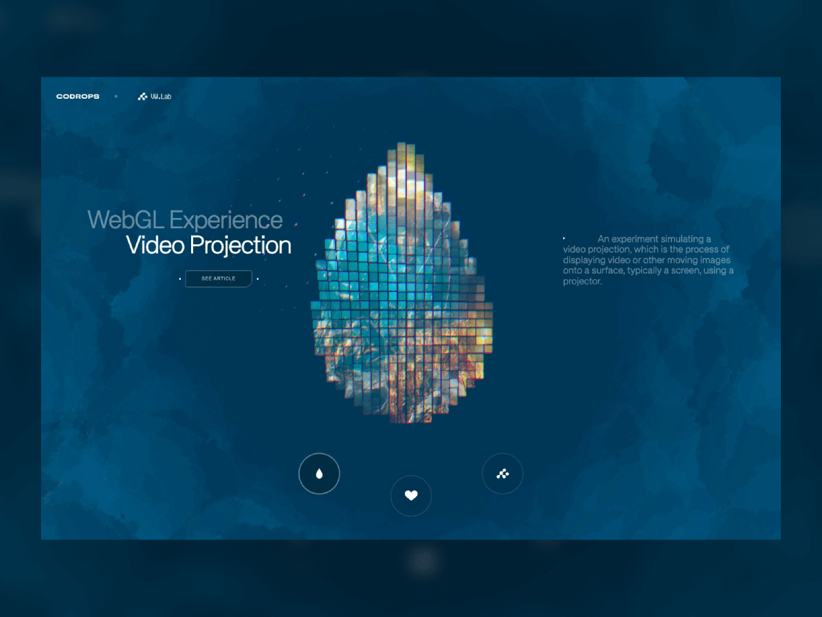
Projection mapping has long fascinated audiences in the physical world, turning buildings, sculptures, and entire cityscapes into moving canvases. What if you could recreate that same sense of spectacle directly inside the browser?

With WebGL and Three.js, you can project video not onto walls or monuments but onto dynamic 3D grids made of hundreds of cubes, each one carrying a fragment of the video like a digital mosaic. Many will surely recognize this effect from Rogier de Boevé’s portfolio, which gained wide attention for showcasing exactly this approach.

In this tutorial we’ll explore how to simulate video projection mapping in a purely digital environment, from building a grid of cubes, to UV-mapping video textures, to applying masks that determine which cubes appear. The demo for this tutorial is inspired by Rogier’s work, which he breaks down beautifully in his case study for anyone interested in the concept behind it.

The result is a mesmerizing effect that feels both sculptural and cinematic, perfect for interactive installations, portfolio showcases, or simply as a playground to push your creative coding skills further.

What is Video Projection Mapping in the Real World?

When describing video projection mapping, it’s easiest to think of huge buildings lit up with animations during festivals, or art installations where a moving image is “painted” onto sculptures.

Here are some examples of real-world video projections:

Bringing it to our 3D World

In 3D graphics, we can do something similar: instead of shining a physical projector, we map a video texture onto objects in a scene.

Therefore, let’s build a grid of cubes using a mask image that will determine which cubes are visible. A video texture is UV-mapped so each cube shows the exact video fragment that corresponds to its grid cell—together they reconstruct the video, but only where the mask is dark.

Prerequesites:

• Three.js r155+
• A small, high-contrast mask image (e.g. a heart silhouette).
• A video URL with CORS enabled.

Our Boilerplate and Starting Point

Here is a basic starter setup, i.e. the minimum amount of code and structure you need to get a scene rendering in the browser, without worrying about the specific creative content yet.

export default class Models {
	constructor(gl_app) {
        ...
        this.createGrid()
    }

    createGrid() {
        const geometry = new THREE.BoxGeometry( 1, 1, 1 );
        this.material = new THREE.MeshStandardMaterial( { color: 0xff0000 } );
        const cube = new THREE.Mesh( geometry, this.material );
        this.group.add( cube );
        this.is_ready = true
    }
    
    ...
}

The result is a spinning red cube:

Creating the Grid

A centered grid of cubes (10×10 by default). Every cube has the same size and material. The grid spacing and overall scale are configurable.

export default class Models {
	constructor(gl_app) {
        ...

		this.gridSize = 10;
        this.spacing = 0.75;
        this.createGrid()
    }

    createGrid() {
        this.material = new THREE.MeshStandardMaterial( { color: 0xff0000 } );
        
        // Grid parameters
        for (let x = 0; x < this.gridSize; x++) {
            for (let y = 0; y < this.gridSize; y++) {
                const geometry = new THREE.BoxGeometry(0.5, 0.5, 0.5);
                const mesh = new THREE.Mesh(geometry, this.material);
                mesh.position.x = (x - (this.gridSize - 1) / 2) * this.spacing;
                mesh.position.y = (y - (this.gridSize - 1) / 2) * this.spacing;
                mesh.position.z = 0;

                this.group.add(mesh);
            }
        }
        this.group.scale.setScalar(0.5)
        ...
    }   
    ...
}

Key parameters

World-space distance between cube centers. Increase for larger gaps, decrease to pack tighter.

How many cells per side. A 10×10 grid ⇒ 100 cubes

Creating the Video Texture

This function creates a video texture in Three.js so you can use a playing HTML <video> as the texture on 3D objects.

• Creates an HTML <video> element entirely in JavaScript (not added to the DOM).
• We’ll feed this element to Three.js to use its frames as a texture.
• loop = true → restarts automatically when it reaches the end.
• muted = true → most browsers block autoplay for unmuted videos, so muting ensures it plays without user interaction.
• .play() → starts playback.
• ⚠️ Some browsers still need a click/touch before autoplay works — you can add a fallback listener if needed.

export default class Models {
	constructor(gl_app) {
        ...
        this.createGrid()
    }

    createVideoTexture() {
		this.video = document.createElement('video')
		this.video.src = 'https://commondatastorage.googleapis.com/gtv-videos-bucket/sample/BigBuckBunny.mp4'
		this.video.crossOrigin = 'anonymous'
		this.video.loop = true
		this.video.muted = true
		this.video.play()

		// Create video texture
		this.videoTexture = new THREE.VideoTexture(this.video)
		this.videoTexture.minFilter = THREE.LinearFilter
		this.videoTexture.magFilter = THREE.LinearFilter
		this.videoTexture.colorSpace = THREE.SRGBColorSpace
		this.videoTexture.wrapS = THREE.ClampToEdgeWrap
		this.videoTexture.wrapT = THREE.ClampToEdgeWrap

		// Create material with video texture
		this.material = new THREE.MeshBasicMaterial({ 
			map: this.videoTexture,
			side: THREE.FrontSide
		})
    }

    createGrid() {
        this.createVideoTexture()
        ...
    }
    ...
}

This is the video we are using: Big Buck Bunny (without CORS)

All the meshes have the same texture applied:

Attributing Projection to the Grid

We will be turning the video into a texture atlas split into a gridSize × gridSize lattice.
Each cube in the grid gets its own little UV window (sub-rectangle) of the video so, together, all cubes reconstruct the full frame.

Why per-cube geometry? Because we can create a new BoxGeometry for each cube since the UVs must be unique per cube. If all cubes shared one geometry, they’d also share the same UVs and show the same part of the video.

export default class Models {
	constructor(gl_app) {
        ...
        this.createGrid()
    }

    createGrid() {
        ...
		// Grid parameters
        for (let x = 0; x < this.gridSize; x++) {
            for (let y = 0; y < this.gridSize; y++) {
                
                const geometry = new THREE.BoxGeometry(0.5, 0.5, 0.5);
                
				// Create individual geometry for each box to have unique UV mapping
				// Calculate UV coordinates for this specific box
				const uvX = x / this.gridSize
				const uvY = y / this.gridSize // Remove the flip to match correct orientation
				const uvWidth = 1 / this.gridSize
				const uvHeight = 1 / this.gridSize
				
				// Get the UV attribute
				const uvAttribute = geometry.attributes.uv
				const uvArray = uvAttribute.array
				
				// Map each face of the box to show the same portion of video
				// We'll focus on the front face (face 4) for the main projection
				for (let i = 0; i < uvArray.length; i += 2) {
					// Map all faces to the same UV region for consistency
					uvArray[i] = uvX + (uvArray[i] * uvWidth)     // U coordinate
					uvArray[i + 1] = uvY + (uvArray[i + 1] * uvHeight) // V coordinate
				}
				
				// Mark the attribute as needing update
				uvAttribute.needsUpdate = true
                ...
            }
        }
        ...
    }
    ...
}

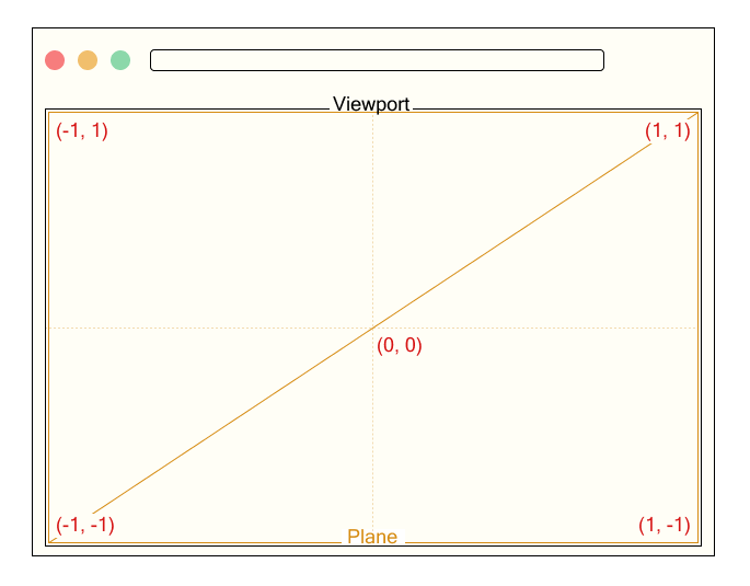
The UV window for cell (x, y)
For a grid of size N = gridSize:

• UV origin of this cell:
  – uvX = x / N
  – uvY = y / N
• UV size of each cell:
  – uvWidth = 1 / N
  – uvHeight = 1 / N

Result: every face of the box now samples the same sub-region of the video (and we noted “focus on the front face”; this approach maps all faces to that region for consistency).

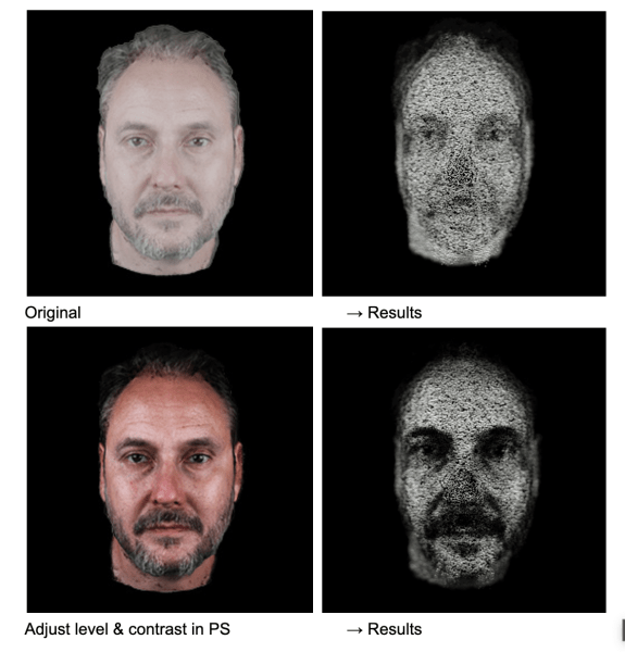
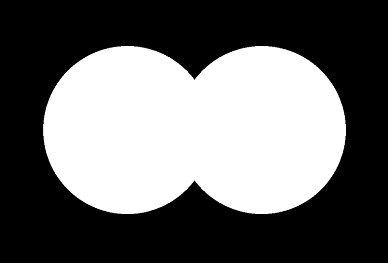
Creating Mask

We need to create a canvas using a mask that determines which cubes are visible in the grid.

• Black (dark) pixels → cube is created.
• White (light) pixels → cube is skipped.

To do this, we need to:

1. Load the mask image.
2. Scale it down to match our grid size.
3. Read its pixel color data.
4. Pass that data into the grid-building step.

export default class Models {
	constructor(gl_app) {
        ...
		this.createMask()
    }

	createMask() {
        // Create a canvas to read mask pixel data
        const canvas = document.createElement('canvas')
        const ctx = canvas.getContext('2d')

        const maskImage = new Image()
        maskImage.crossOrigin = 'anonymous'
        maskImage.onload = () => {
            // Get original image dimensions to preserve aspect ratio
            const originalWidth = maskImage.width
            const originalHeight = maskImage.height
            const aspectRatio = originalWidth / originalHeight

            // Calculate grid dimensions based on aspect ratio
            this.gridWidth
			this.gridHeight
            if (aspectRatio > 1) {
                // Image is wider than tall
                this.gridWidth = this.gridSize
                this.gridHeight = Math.round(this.gridSize / aspectRatio)
            } else {
                // Image is taller than wide or square
                this.gridHeight = this.gridSize
                this.gridWidth = Math.round(this.gridSize * aspectRatio)
            }

            canvas.width = this.gridWidth
            canvas.height = this.gridHeight
            ctx.drawImage(maskImage, 0, 0, this.gridWidth, this.gridHeight)

            const imageData = ctx.getImageData(0, 0, this.gridWidth, this.gridHeight)
            this.data = imageData.data
			this.createGrid()
		}

        maskImage.src = '../images/heart.jpg'
	}
    ...
}

Match mask resolution to grid

• We don’t want to stretch the mask — this keeps it proportional to the grid.
• gridWidth and gridHeight are how many mask pixels we’ll sample horizontally and vertically.
• This matches the logical cube grid, so each cube can correspond to one pixel in the mask.

Applying the Mask to the Grid

Let’s combines mask-based filtering with custom UV mapping to decide where in the grid boxes should appear, and how each box maps to a section of the projected video.
Here’s the concept step by step:

• Loops through every potential (x, y) position in a virtual grid.
• At each grid cell, it will decide whether to place a box and, if so, how to texture it.
• flippedY: Flips the Y-axis because image coordinates start from the top-left, while the grid’s origin starts from the bottom-left.
• pixelIndex: Locates the pixel in the this.data array.
• Each pixel stores 4 values: red, green, blue, alpha.
• Extracts the R, G, and B values for that mask pixel.
• Brightness is calculated as the average of R, G, B.
• If the pixel is dark enough (brightness < 128), a cube will be created.
• White pixels are ignored → those positions stay empty.

export default class Models {
	constructor(gl_app) {
        ...
		this.createMask()
    }

	createMask() {
        ...
	}

    createGrid() {
        ...
        for (let x = 0; x < this.gridSize; x++) {
            for (let y = 0; y < this.gridSize; y++) {
                
                const geometry = new THREE.BoxGeometry(0.5, 0.5, 0.5);

                // Get pixel color from mask (sample at grid position)
                // Flip Y coordinate to match image orientation
                const flippedY = this.gridHeight - 1 - y
                const pixelIndex = (flippedY * this.gridWidth + x) * 4
                const r = this.data[pixelIndex]
                const g = this.data[pixelIndex + 1]
                const b = this.data[pixelIndex + 2]

                // Calculate brightness (0 = black, 255 = white)
                const brightness = (r + g + b) / 3

                // Only create box if pixel is dark (black shows, white hides)
                if (brightness < 128) { // Threshold for black vs white

                    // Create individual geometry for each box to have unique UV mapping
                    // Calculate UV coordinates for this specific box
                    const uvX = x / this.gridSize
                    const uvY = y / this.gridSize // Remove the flip to match correct orientation
                    const uvWidth = 1 / this.gridSize
                    const uvHeight = 1 / this.gridSize
                    
                    // Get the UV attribute
                    const uvAttribute = geometry.attributes.uv
                    const uvArray = uvAttribute.array
                    
                    // Map each face of the box to show the same portion of video
                    // We'll focus on the front face (face 4) for the main projection
                    for (let i = 0; i < uvArray.length; i += 2) {
                        // Map all faces to the same UV region for consistency
                        uvArray[i] = uvX + (uvArray[i] * uvWidth)     // U coordinate
                        uvArray[i + 1] = uvY + (uvArray[i + 1] * uvHeight) // V coordinate
                    }
                    
                    // Mark the attribute as needing update
                    uvAttribute.needsUpdate = true
                    
                    const mesh = new THREE.Mesh(geometry, this.material);

                    mesh.position.x = (x - (this.gridSize - 1) / 2) * this.spacing;
                    mesh.position.y = (y - (this.gridSize - 1) / 2) * this.spacing;
                    mesh.position.z = 0;

                    this.group.add(mesh);
                }
            }
        }
        ...
    }
    ...
}

Further steps

• UV mapping is the process of mapping 2D video pixels onto 3D geometry.
• Each cube gets its own unique UV coordinates corresponding to its position in the grid.
• uvWidth and uvHeight are how much of the video texture each cube covers.
• Modifies the cube’s uv attribute so all faces display the exact same portion of the video.

Here is the result with the mask applied:

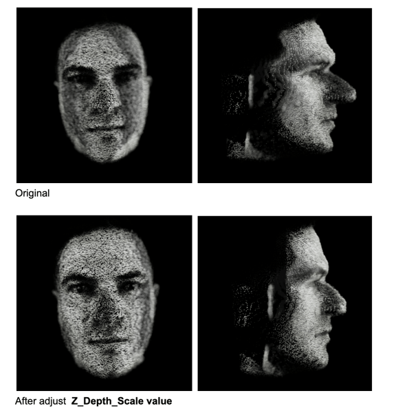
Adding Some Depth and Motion to the Grid

Adding subtle motion along the Z-axis brings the otherwise static grid to life, making the projection feel more dynamic and dimensional.

update() {
    if (this.is_ready) {
        this.group.children.forEach((model, index) => {
            model.position.z = Math.sin(Date.now() * 0.005 + index * 0.1) * 0.6
        })
    }
}

It’s the time for Multiple Grids

Up until now we’ve been working with a single mask and a single video, but the real fun begins when we start layering multiple projections together. By combining different mask images with their own video sources, we can create a collection of independent grids that coexist in the same scene. Each grid can carry its own identity and motion, opening the door to richer compositions, transitions, and storytelling effects.

1. A Playlist of Masks and Videos

export default class Models {
	constructor(gl_app) {
        ...
        this.grids_config = [
            {
                id: 'heart',
                mask: `heart.jpg`,
                video: `fruits_trail_squared-transcode.mp4`
            },
            {
                id: 'codrops',
                mask: `codrops.jpg`,
                video: `KinectCube_1350-transcode.mp4`
            },
            {
                id: 'smile',
                mask: `smile.jpg`,
                video: `infinte-grid_squared-transcode.mp4`
            },
        ]
        this.grids_config.forEach((config, index) => this.createMask(config, index))
        this.grids = []
    }
...
}

Instead of one mask and one video, we now have a list of mask-video pairs.

Each object defines:

• id → name/id for each grid.
• mask → the black/white image that controls which cubes appear.
• video → the texture that will be mapped onto those cubes.

This allows you to have multiple different projections in the same scene.

2. Looping Over All Grids

Once we have our playlist of mask–video pairs defined, the next step is to go through each item and prepare it for rendering.

For every configuration in the list we call createMask(config, index), which takes care of loading the mask image, reading its pixels, and then passing the data along to build the corresponding grid.

At the same time, we keep track of all the grids by storing them in a this.grids array, so later on we can animate them, show or hide them, and switch between them interactively.

3. createMask(config, index)

createMask(config, index) {
    ...
    maskImage.onload = () => {
        ...
        this.createGrid(config, index)
    }
    maskImage.src = `../images/${config.mask}`
}

• Loads the mask image for the current grid.
• When the image is loaded, runs the mask pixel-reading logic (as explained before) and then calls createGrid() with the same config and index.
• The mask determines which cubes are visible for this specific grid.

4. createVideoTexture(config, index)

createVideoTexture(config, index) {
    this.video = document.createElement('video')
    this.video.src = `../videos/${config.video}`
    ...
}

• Creates a <video> element using the specific video file for this grid.
• The video is then converted to a THREE.VideoTexture and assigned as the material for the cubes in this grid.
• Each grid can have its own independent video playing.

5. createGrid(config, index)

createGrid(config, index) {
        this.createVideoTexture(config, index)
        const grid_group = new THREE.Group()
        this.group.add(grid_group)

        for (let x = 0; x < this.gridSize; x++) {
            for (let y = 0; y < this.gridSize; y++) {
                    ...
                    grid_group.add(mesh);
            }
        }
        grid_group.name = config.id
        this.grids.push(grid_group);
        grid_group.position.z = - 2 * index 
        ...
    }

• Creates a new THREE.Group for this grid so all its cubes can be moved together.
• This keeps each mask/video projection isolated.
• grid_group.name: Assigns a name (you might later use config.id here).
• this.grids.push(grid_group): Stores this grid in an array so you can control it later (e.g., show/hide, animate, change videos).
• grid_group.position.z: Offsets each grid further back in Z-space so they don’t overlap visually.

And here is the result for the multiple grids:

And finally: Interaction & Animations

Let’s start by creating a simple UI with some buttons on our HTML:

<ul class="btns">
	<li class="btns__item">
		<button class="active" data-id="heart">
			...
		</button>
	</li>
	<li class="btns__item">
		<button data-id="codrops">
			...
		</button>
	</li>
	<li class="btns__item">
		<button data-id="smile">
			...
		</button>
	</li>
</ul>

We’ll also create a data-current="heart" to our canvas element, it will be necessary to change its background-color depending on which button was clicked.

<canvas id="sketch" data-current="heart"></canvas>

Let’s not create some colors for each grid using CSS:

[data-current="heart"] {
	background-color: #e19800;
}

[data-current="codrops"] {
	background-color: #00a00b
}

[data-current="smile"] {
	background-color: #b90000;
}

Time to apply to create the interactions:

createGrid(config, index) {
    ...
    this.initInteractions()
}

1. this.initInteractions()

initInteractions() {
    this.current = 'heart'
    this.old = null
    this.is_animating = false
    this.duration = 1

    this.DOM = {
        $btns: document.querySelectorAll('.btns__item button'),
        $canvas: document.querySelector('canvas')
    }
    this.grids.forEach(grid => {
        if(grid.name != this.current) {
            grid.children.forEach(mesh => mesh.scale.setScalar(0))
        }
    })
    this.bindEvents()
}

• this.current → The currently active grid ID. Starts as "heart" so the "heart" grid will be visible by default.
• this.old → Used to store the previous grid ID when switching between grids.
• this.is_animating → Boolean flag to prevent triggering a new transition while one is still running.
• this.duration → How long the animation takes (in seconds).
• $btns → Selects all the buttons inside .btns__item. Each button likely corresponds to a grid you can switch to.
• $canvas → Selects the main <canvas> element where the Three.js scene is rendered.

Loops through all the grids in the scene.

• If the grid is not the current one (grid.name != this.current),
• → It sets all of that grid’s cubes (mesh) to scale = 0 so they are invisible at the start.
• This means only the "heart" grid will be visible when the scene first loads.

2. bindEvents()

bindEvents() {
    this.DOM.$btns.forEach(($btn, index) => {
        $btn.addEventListener('click', () => {
            if (this.is_animating) return
            this.is_animating = true
            this.DOM.$btns.forEach(($btn, btnIndex) => {
                btnIndex === index ? $btn.classList.add('active') : $btn.classList.remove('active')
            })
            this.old = this.current
            this.current = `${$btn.dataset.id}`
            this.revealGrid()
            this.hideGrid()
        })
    })
}

This bindEvents() method wires up the UI buttons so that clicking one will trigger switching between grids in the 3D scene.

• For each button, attach a click event handler.
• If an animation is already running, do nothing — this prevents starting multiple transitions at the same time.
• Sets is_animating to true so no other clicks are processed until the current switch finishes.

Loops through all buttons again:

• If this is the clicked button → add the active CSS class (highlight it).
• Otherwise → remove the active class (unhighlight).
• this.old → keeps track of which grid was visible before the click.
• this.current → updates to the new grid’s ID based on the button’s data-id attribute.
  • Example: if the button has data-id="heart", this.current becomes "heart".

Calls two separate methods:

• revealGrid() → makes the newly selected grid appear (by scaling its cubes from 0 to full size).
• hideGrid() → hides the previous grid (by scaling its cubes back down to 0).

3. revealGrid() & hideGrid()

revealGrid() {
    // Filter the current grid based on this.current value
    const grid = this.grids.find(item => item.name === this.current);
    
    this.DOM.$canvas.dataset.current = `${this.current}` 
    const tl = gsap.timeline({ delay: this.duration * 0.25, defaults: { ease: 'power1.out', duration: this.duration } })
    grid.children.forEach((child, index) => {
        tl
            .to(child.scale, { x: 1, y: 1, z: 1, ease: 'power3.inOut' }, index * 0.001)
            .to(child.position, { z: 0 }, '<')
    })
}

hideGrid() {
    // Filter the current grid based on this.old value
    const grid = this.grids.find(item => item.name === this.old);
    const tl = gsap.timeline({
        defaults: { ease: 'power1.out', duration: this.duration },
        onComplete: () => { this.is_animating = false }
    })
    grid.children.forEach((child, index) => {
        tl
            .to(child.scale, { x: 0, y: 0, z: 0, ease: 'power3.inOut' }, index * 0.001)
            .to(child.position, {
                z: 6, onComplete: () => {
                    gsap.set(child.scale, { x: 0, y: 0, z: 0 })
                    gsap.set(child.position, { z: - 6 })
                }
            }, '<')
    })
}

And that is it! A full animated and interactive Video Projection Slider, made with hundreds of small cubes (meshes).

⚠️ Perfomance considerations

The approach used in this tutorial, is the simplest and more digestable way to apply the projection concept; However, it can create too many draw calls: 100–1,000 cubes might fine; tens of thousands can be slow. If you need more detailed grid or more meshes on it, consider InstancedMesh and Shaders.

Going further

This a fully functional and versatile concept; Therefore, it opens so many possibilities.
Which can be applied in some really cool ways, like scrollable story-telling, exhibition simulation, intro animations, portfolio showcase and etc.

Here are some links for you to get inspired:

Final Words

I hope you’ve enjoyed this tutorial, and give a try on your projects or just explore the possibilities by changing the grid parameters, masks and videos.

And talking about the videos, those used on this example are screen-recording of the Creative Code lessons contained in my Web Animations platform vwlab.io, where you can learn how to create more interactions and animations like this one.

Come join us, you will be more than welcome! ☺️❤️