When working with data, you will often move between SQL databases and Pandas DataFrames. SQL is excellent for storing and retrieving data, while Pandas is ideal for analysis inside Python.
In this article, we show how both can be used together, using a football (soccer) mini-league dataset. We build a small SQLite database in memory, read the data into Pandas, and then solve real analytics questions.

There are neither pythons or pandas in Bulgaria. Just software.
-
Setup – SQLite and Pandas
We start by importing the libraries and creating three tables –
[teams, players, matches] inside an SQLite in-memory database.
1
2
3
4
5
6
7
8
9
10
11
12
13
14
15
16
17
18
19
20
21
22
23
24
25
26
27
28
29
30
31
32
33
34
35
36
37
38
39
40
41
42
43
44
45
46
47
48
49
50
51
52
53
54
55
56
57
|
import sqlite3
import pandas as pd
import numpy as np
conn = sqlite3.connect(“:memory:”)
cur = conn.cursor()
cur.executescript(“””
DROP TABLE IF EXISTS teams;
DROP TABLE IF EXISTS players;
DROP TABLE IF EXISTS matches;
CREATE TABLE teams (
team TEXT PRIMARY KEY,
city TEXT NOT NULL,
founded INTEGER NOT NULL
);
CREATE TABLE players (
player_id INTEGER PRIMARY KEY AUTOINCREMENT,
name TEXT NOT NULL,
team TEXT NOT NULL REFERENCES teams(team),
pos TEXT NOT NULL,
age INTEGER NOT NULL,
goals INTEGER NOT NULL,
assists INTEGER,
minutes INTEGER NOT NULL
);
CREATE TABLE matches (
match_id INTEGER PRIMARY KEY AUTOINCREMENT,
date TEXT NOT NULL,
home TEXT NOT NULL,
away TEXT NOT NULL,
home_goals INTEGER NOT NULL,
away_goals INTEGER NOT NULL
);
INSERT INTO teams(team, city, founded) VALUES
(‘Lions’,’Sofia’, 2015),
(‘Wolves’,’Plovdiv’,1914),
(‘Eagles’,’Varna’,1930);
INSERT INTO players(name, team, pos, age, goals, assists, minutes) VALUES
(‘Ivan Petrov’,’Lions’,’FW’,24,11,3,1350),
(‘Martin Kolev’,’Lions’,’MF’,29,4,NULL,1490),
(‘Rui Costa’,’Lions’,’DF’,31,1,2,1600),
(‘Georgi Iliev’,’Wolves’,’FW’,27,7,5,1410),
(‘Joe Jackson’,’Wolves’,’FW’,27,17,5,410),
(‘Peter Marin’,’Eagles’,’FW’,20,5,1,870);
INSERT INTO matches(date,home,away,home_goals,away_goals) VALUES
(‘2024-08-03′,’Lions’,’Wolves’,2,1),
(‘2024-08-10′,’Eagles’,’Lions’,1,3),
(‘2024-08-17′,’Wolves’,’Eagles’,2,2);
“””)
conn.commit()
|
Now, we have three tables.
-
Loading SQL Data into Pandas
pd.read_sql does the magic to load either a table or a custom query directly.
|
teams = pd.read_sql(“SELECT * FROM teams”, conn)
players = pd.read_sql(“SELECT * FROM players”, conn)
matches = pd.read_sql(“SELECT * FROM matches”, conn, parse_dates = [“date”])
print(teams)
print(players.head())
print(matches)
|
At this point, the SQL data is ready for analysis with Pandas.
-
SQL vs Pandas – Filtering Rows
Task: Find forwards (FW) with more than 1200 minutes on the field:
SQL:
|
sql1 = pd.read_sql(“””
SELECT name, team, goals
FROM players
WHERE pos=”FW” AND minutes > 1200;
“””, conn)
|
Pandas:
|
pd1 = players.loc[(players[‘pos’]==‘FW’)&(players[“minutes”]>1200),[“name”, “team”, “goals”]]
|
As expected, both return the same subset, one written in SQL and the other in Pandas.
Task: Total goals per team:
SQL:
|
sql2 = pd.read_sql(“””
SELECT team, SUM(goals)
FROM players
GROUP BY team
ORDER BY 2 DESC;
“””, conn)
|
Pandas:
|
pd2 = players.groupby(“team”)[“goals”].sum().reset_index()
pd2.sort_values(“goals”, ascending = False).reset_index(drop=True)
|
Both results show which team has scored more goals overall.
Task: Add the city of each team to the players table.
SQL:
|
sql3 = pd.read_sql(“””
SELECT p.name, t.city
FROM players p
JOIN teams t on t.team = p.team;
“””, conn)
|
Pandas:
|
pd3 = players.merge(teams, on=“team”, how=“left”)
pd3[[“name”, “city”]]
|
The fun part: calculating points (3 for a win, 1 for a draw) and goal difference. Only with SQL this time.
|
m[“home_points”] = np.where(m[“home_goals”]>m[“away_goals”],3,
np.where(m[“home_goals”]==m[“away_goals”],1,0))
m[“away_points”] = np.where(m[“away_goals”]>m[“home_goals”],3,
np.where(m[“away_goals”]==m[“home_goals”],1,0))
home_tbl = m[[“home”,“home_points”,“home_goals”,“away_goals”]] \
.rename(columns={“home”:“team”,“home_points”:“points”,“home_goals”:“gf”,“away_goals”:“ga”})
away_tbl = m[[“away”,“away_points”,“away_goals”,“home_goals”]] \
.rename(columns={“away”:“team”,“away_points”:“points”,“away_goals”:“gf”,“home_goals”:“ga”})
total_points = pd.concat([home_tbl,away_tbl])
league = total_points.groupby(“team”).agg(points=(“points”,“sum”), GF=(“gf”,“sum”), GA=(“ga”,“sum”))
league[“GD”] = league[“GF”] – league[“GA”]
league.sort_values([“points”,“GD”], ascending=[False,False])
|
This produces a proper football league ranking – teams sorted by points and then goal difference:

-
Quick Pandas Tricks
- Top scorers with
nlargest:
|
pd4 = players.nlargest(3, “goals”)
pd4 = pd4[[“name”, “team”, “goals”]]
pd4
|
|
bins = [0, 22, 26, 30, np.inf]
labels = [“<=22”, “23-26”, “27-30”, “31+”]
players[“age_band”] = pd.cut(players[“age”], bins = bins, labels = labels)
|
https://www.youtube.com/watch?v=U0lbBaHFAEM
https://github.com/Vitosh/Python_personal/tree/master/YouTube/041_Python-Learn-Pandas-with-Football-Analytics