Every project begins with a spark of curiosity. It often emerges from exploring techniques outside the web and imagining how they might translate into interactive experiences. In this case, inspiration came from a dive into particle simulations.
The Concept
The core idea for this project came after watching a tutorial on creating cell-like particles using the xParticles plugin for Cinema 4D. The team often draws inspiration from 3D motion design techniques, and the question frequently arises in the studio: “Wouldn’t this be cool if it were interactive?” That’s where the idea was born.
After building our own set up in C4D based on the example, we created a general motion prototype to demonstrate the interaction. The result was a kind of repelling effect, where the cells displaced according to the cursor’s position. To create the demo, we added a simple sphere and gave it a collider tag so that the particles would be pushed away as the sphere moved through the simulation, emulating the mouse movement. An easy way to add realistic movement is to add a vibrate tag to the collider, and play around with the movement levels and frequency until it looks good.
Art Direction
With the base particle and interaction demo sorted, we rendered out the sequence and moved in After Effects to start playing around with the look and feel. We knew we wanted to give the particles a unique quality, one that felt more stylised as opposed to ultra realistic or scientific. After some exploration we landed on a lo-fi gradient mapped look, which felt like an interesting direction to move forward with. We achieved this by layer up a few effects:
Effect > Generate > 4 Colour Gradient: Add this to a new shape layer. This black and white gradient will act as a mask to control the blur intensities.
Effect > Blur > Camera Blur: Add this to a new adjustment layer. This general blur will smooth out the particles.
Effect > Blur > Compound Blur: Add this to the same adjustment layer as above. Set the blur layer to use the same shape layer we applied to the 4 colour gradient as its mask, make sure it is set to “Effects & Mask” mode in the drop down.
Effect > Color Correction > Colorama: Add this as a new adjustment layer. This is where the fun starts! You can add custom gradients into the output cycle and play around with the phase shift to customise the look according to your preference.
Next, we designed a simple UI to match the futuristic cell-based visual direction. A concept we felt would work well for a bio-tech company – so created a simple brand with key messaging to fit and voila! That’s the concept phase complete.
(Hot tip: If you’re doing an interaction concept in 3d software like C4D, create a plane with a cursor texture on and parent it to your main interaction component – in the case, the sphere collider. Render that out as a sequence so that it matches up perfectly with your simulation – you can then layer it over text, etc, and UI in After Effects)
Technical Approach and Tools
As this was a simple one page static site without need of a backend, we used our in-house boilerplate using Astro with Vite and Three.js. For the physics, we went with Rapier as it handles collision detection efficiently and is compatible with Three.js. That was our main requirement, since we didn’t need simulations or soft-body calculations.
For the Cellular Technology project, we specifically wanted to show how you can achieve a satisfying result without overcrowding the screen with tons of features or components. Our key focus was the visuals and interactivity – to make this satisfying for the user, it needed to feel smooth and seamless. A fluid-like simulation is a good way to achieve this. At Unseen, we often implement this effect as an added interaction component. For this project, we wanted to take a slightly different approach that would still achieve a similar result.
Based on the concept from our designers, there were a couple of directions for the implementation to consider. To keep the experience optimised, even at a large scale, having the GPU handle the majority of the calculations is usually the best approach. For this, we’d need the effect to be in a shader, and use more complicated implementations such as packing algorithms and custom voronoi-like patterns. However, after testing the Rapier library, we realised that simple rigid body object collision would suffice in re-creating the concept in real-time.
Physics Implementation
To do so, we needed to create a separate physics world next to our 3D rendered world, as the Rapier library only handles the physics calculations, and the graphics are left for the implementation of the developer’s choosing.
Here’s a snippet from the part were we create the rigid bodies:
for (let i = 0; i < this.numberOfBodies; i++) {
  const x = Math.random() * this.bounds.x - this.bounds.x * 0.5
  const y = Math.random() * this.bounds.y - this.bounds.y * 0.5
  const z = Math.random() * (this.bounds.z * 0.95) - (this.bounds.z * 0.95) * 0.5

  const bodyDesc = RAPIER.RigidBodyDesc.dynamic().setTranslation(x, y, z)
  bodyDesc.setGravityScale(0.0) // Disable gravity
  bodyDesc.setLinearDamping(0.7)
  const body = this.physicsWorld.createRigidBody(bodyDesc)

  const radius = MathUtils.mapLinear(Math.random(), 0.0, 1.0, this._cellSizeRange[0], this._cellSizeRange[1])
  const colliderDesc = RAPIER.ColliderDesc.ball(radius)
  const collider = this.physicsWorld.createCollider(colliderDesc, body)
  collider.setRestitution(0.1) // bounciness 0 = no bounce, 1 = full bounce

  this.bodies.push(body)
  this.colliders.push(collider)
}
The meshes that represent the bodies are created separately, and on each tick, their transforms get updated by those from the physics engine.
// update mesh positions
for (let i = 0; i < this.numberOfBodies; i++) {
  const body = this.bodies[i]
  const position = body.translation()

  const collider = this.colliders[i]
  const radius = collider.shape.radius

  this._dummy.position.set(position.x, position.y, position.z)
  this._dummy.scale.setScalar(radius)
  this._dummy.updateMatrix()

  this.mesh.setMatrixAt(i, this._dummy.matrix)
}

this.mesh.instanceMatrix.needsUpdate = true
With performance in mind, we first decided to try the 2D version of the Rapier library, however it soon became clear that with cells distributed only in one plane, the visual was not convincing enough. The performance impact of additional calculations in the Z plane was justified by the improved result.
Building the Visual with Post Processing
Evidently, the post processing effects play a big role in this project. By far the most important is the blur, which makes the cells go from clear simple rings to a fluid, gooey mass. We implemented the Kawase blur, which is similar to Gaussian blur, but uses box blurring instead of the Gaussian function and is more performant at higher levels of blur. We applied it to only some parts of the screen to keep visual interest.
This already brought the implementation closer to the concept. Another vital part of the experience is the color-grading, where we mapped the colours to the luminosity of elements in the scene. We couldn’t resist adding our typical fluid simulation, so the colours get slightly offset based on the fluid movement.
if (uFluidEnabled) {
    fluidColor = texture2D(tFluid, screenCoords);

    fluid = pow(luminance(abs(fluidColor.rgb)), 1.2);
    fluid *= 0.28;
}

vec3 color1 = uColor1 - fluid * 0.08;
vec3 color2 = uColor2 - fluid * 0.08;
vec3 color3 = uColor3 - fluid * 0.08;
vec3 color4 = uColor4 - fluid * 0.08;

if (uEnabled) {
    // apply a color grade
    color = getColorRampColor(brightness, uStops.x, uStops.y, uStops.z, uStops.w, color1, color2, color3, color4);
}

color += color * fluid * 1.5;
color = clamp(color, 0.0, 1.0);

color += color * fluidColor.rgb * 0.09;

gl_FragColor = vec4(color, 1.0);
Performance Optimisation
With the computational power required for the physics engine increasing quickly due to the number of calculations required, we aimed to make the experience as optimised as possible. The first step was to find the minimum number of cells without affecting the visual too much, i.e. without making the cells too sparse. To do so, we minimised the area in which the cells get created and made the cells slightly larger.
Another important step was to make sure no calculation is redundant, meaning each calculation must be justified by a result visible on the screen. To make sure of that, we limited the area in which cells get created to only just cover the screen, regardless of the screen size. This basically means that all cells in the scene are visible in the camera. Usually this approach involves a slightly more complex derivation of the bounding area, based on the camera field of view and distance from the object, however, for this project, we used an orthographic camera, which simplifies the calculations.
Projection mapping has long fascinated audiences in the physical world, turning buildings, sculptures, and entire cityscapes into moving canvases. What if you could recreate that same sense of spectacle directly inside the browser?
With WebGL and Three.js, you can project video not onto walls or monuments but onto dynamic 3D grids made of hundreds of cubes, each one carrying a fragment of the video like a digital mosaic. Many will surely recognize this effect from Rogier de Boevé’s portfolio, which gained wide attention for showcasing exactly this approach.
In this tutorial we’ll explore how to simulate video projection mapping in a purely digital environment, from building a grid of cubes, to UV-mapping video textures, to applying masks that determine which cubes appear. The demo for this tutorial is inspired by Rogier’s work, which he breaks down beautifully in his case study for anyone interested in the concept behind it.
The result is a mesmerizing effect that feels both sculptural and cinematic, perfect for interactive installations, portfolio showcases, or simply as a playground to push your creative coding skills further.
What is Video Projection Mapping in the Real World?
When describing video projection mapping, it’s easiest to think of huge buildings lit up with animations during festivals, or art installations where a moving image is “painted” onto sculptures.
Here are some examples of real-world video projections:
Bringing it to our 3D World
In 3D graphics, we can do something similar: instead of shining a physical projector, we map a video texture onto objects in a scene.
Therefore, let’s build a grid of cubes using a mask image that will determine which cubes are visible. A video texture is UV-mapped so each cube shows the exact video fragment that corresponds to its grid cell—together they reconstruct the video, but only where the mask is dark.
Prerequesites:
Three.js r155+
A small, high-contrast mask image (e.g. a heart silhouette).
A video URL with CORS enabled.
Our Boilerplate and Starting Point
Here is a basic starter setup, i.e. the minimum amount of code and structure you need to get a scene rendering in the browser, without worrying about the specific creative content yet.
This is the video we are using: Big Buck Bunny (without CORS)
All the meshes have the same texture applied:
Attributing Projection to the Grid
We will be turning the video into a texture atlas split into a gridSize × gridSize lattice. Each cube in the grid gets its own little UV window (sub-rectangle) of the video so, together, all cubes reconstruct the full frame.
Why per-cube geometry? Because we can create a new BoxGeometry for each cube since the UVs must be unique per cube. If all cubes shared one geometry, they’d also share the same UVs and show the same part of the video.
export default class Models {
	constructor(gl_app) {
        ...
        this.createGrid()
    }

    createGrid() {
        ...
		// Grid parameters
        for (let x = 0; x < this.gridSize; x++) {
            for (let y = 0; y < this.gridSize; y++) {

                const geometry = new THREE.BoxGeometry(0.5, 0.5, 0.5);

				// Create individual geometry for each box to have unique UV mapping
				// Calculate UV coordinates for this specific box
				const uvX = x / this.gridSize
				const uvY = y / this.gridSize // Remove the flip to match correct orientation
				const uvWidth = 1 / this.gridSize
				const uvHeight = 1 / this.gridSize

				// Get the UV attribute
				const uvAttribute = geometry.attributes.uv
				const uvArray = uvAttribute.array

				// Map each face of the box to show the same portion of video
				// We'll focus on the front face (face 4) for the main projection
				for (let i = 0; i < uvArray.length; i += 2) {
					// Map all faces to the same UV region for consistency
					uvArray[i] = uvX + (uvArray[i] * uvWidth)     // U coordinate
					uvArray[i + 1] = uvY + (uvArray[i + 1] * uvHeight) // V coordinate
				}

				// Mark the attribute as needing update
				uvAttribute.needsUpdate = true
                ...
            }
        }
        ...
    }
    ...
}
The UV window for cell (x, y) For a grid of size N = gridSize:
UV origin of this cell: – uvX = x / N – uvY = y / N
UV size of each cell: – uvWidth = 1 / N – uvHeight = 1 / N
Result: every face of the box now samples the same sub-region of the video (and we noted “focus on the front face”; this approach maps all faces to that region for consistency).
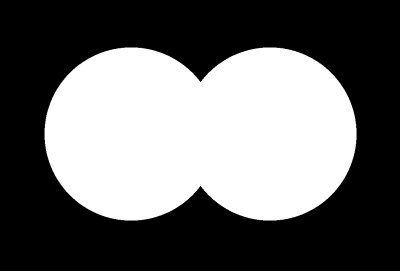
We need to create a canvas using a mask that determines which cubes are visible in the grid.
Black (dark) pixels → cube is created.
White (light) pixels → cube is skipped.
To do this, we need to:
Load the mask image.
Scale it down to match our grid size.
Read its pixel color data.
Pass that data into the grid-building step.
export default class Models {
	constructor(gl_app) {
        ...
		this.createMask()
    }

	createMask() {
        // Create a canvas to read mask pixel data
        const canvas = document.createElement('canvas')
        const ctx = canvas.getContext('2d')

        const maskImage = new Image()
        maskImage.crossOrigin = 'anonymous'
        maskImage.onload = () => {
            // Get original image dimensions to preserve aspect ratio
            const originalWidth = maskImage.width
            const originalHeight = maskImage.height
            const aspectRatio = originalWidth / originalHeight

            // Calculate grid dimensions based on aspect ratio
            this.gridWidth
			this.gridHeight
            if (aspectRatio > 1) {
                // Image is wider than tall
                this.gridWidth = this.gridSize
                this.gridHeight = Math.round(this.gridSize / aspectRatio)
            } else {
                // Image is taller than wide or square
                this.gridHeight = this.gridSize
                this.gridWidth = Math.round(this.gridSize * aspectRatio)
            }

            canvas.width = this.gridWidth
            canvas.height = this.gridHeight
            ctx.drawImage(maskImage, 0, 0, this.gridWidth, this.gridHeight)

            const imageData = ctx.getImageData(0, 0, this.gridWidth, this.gridHeight)
            this.data = imageData.data
			this.createGrid()
		}

        maskImage.src = '../images/heart.jpg'
	}
    ...
}
Match mask resolution to grid
We don’t want to stretch the mask — this keeps it proportional to the grid.
gridWidth and gridHeight are how many mask pixels we’ll sample horizontally and vertically.
This matches the logical cube grid, so each cube can correspond to one pixel in the mask.
Applying the Mask to the Grid
Let’s combines mask-based filtering with custom UV mapping to decide where in the grid boxes should appear, and how each box maps to a section of the projected video. Here’s the concept step by step:
Loops through every potential (x, y) position in a virtual grid.
At each grid cell, it will decide whether to place a box and, if so, how to texture it.
flippedY: Flips the Y-axis because image coordinates start from the top-left, while the grid’s origin starts from the bottom-left.
pixelIndex: Locates the pixel in the this.data array.
Each pixel stores 4 values: red, green, blue, alpha.
Extracts the R, G, and B values for that mask pixel.
Brightness is calculated as the average of R, G, B.
If the pixel is dark enough (brightness < 128), a cube will be created.
White pixels are ignored → those positions stay empty.
export default class Models {
	constructor(gl_app) {
        ...
		this.createMask()
    }

	createMask() {
        ...
	}

    createGrid() {
        ...
        for (let x = 0; x < this.gridSize; x++) {
            for (let y = 0; y < this.gridSize; y++) {

                const geometry = new THREE.BoxGeometry(0.5, 0.5, 0.5);

                // Get pixel color from mask (sample at grid position)
                // Flip Y coordinate to match image orientation
                const flippedY = this.gridHeight - 1 - y
                const pixelIndex = (flippedY * this.gridWidth + x) * 4
                const r = this.data[pixelIndex]
                const g = this.data[pixelIndex + 1]
                const b = this.data[pixelIndex + 2]

                // Calculate brightness (0 = black, 255 = white)
                const brightness = (r + g + b) / 3

                // Only create box if pixel is dark (black shows, white hides)
                if (brightness < 128) { // Threshold for black vs white

                    // Create individual geometry for each box to have unique UV mapping
                    // Calculate UV coordinates for this specific box
                    const uvX = x / this.gridSize
                    const uvY = y / this.gridSize // Remove the flip to match correct orientation
                    const uvWidth = 1 / this.gridSize
                    const uvHeight = 1 / this.gridSize

                    // Get the UV attribute
                    const uvAttribute = geometry.attributes.uv
                    const uvArray = uvAttribute.array

                    // Map each face of the box to show the same portion of video
                    // We'll focus on the front face (face 4) for the main projection
                    for (let i = 0; i < uvArray.length; i += 2) {
                        // Map all faces to the same UV region for consistency
                        uvArray[i] = uvX + (uvArray[i] * uvWidth)     // U coordinate
                        uvArray[i + 1] = uvY + (uvArray[i + 1] * uvHeight) // V coordinate
                    }

                    // Mark the attribute as needing update
                    uvAttribute.needsUpdate = true

                    const mesh = new THREE.Mesh(geometry, this.material);

                    mesh.position.x = (x - (this.gridSize - 1) / 2) * this.spacing;
                    mesh.position.y = (y - (this.gridSize - 1) / 2) * this.spacing;
                    mesh.position.z = 0;

                    this.group.add(mesh);
                }
            }
        }
        ...
    }
    ...
}
Further steps
UV mapping is the process of mapping 2D video pixels onto 3D geometry.
Each cube gets its own unique UV coordinates corresponding to its position in the grid.
uvWidth and uvHeight are how much of the video texture each cube covers.
Modifies the cube’s uv attribute so all faces display the exact same portion of the video.
Up until now we’ve been working with a single mask and a single video, but the real fun begins when we start layering multiple projections together. By combining different mask images with their own video sources, we can create a collection of independent grids that coexist in the same scene. Each grid can carry its own identity and motion, opening the door to richer compositions, transitions, and storytelling effects.
Instead of one mask and one video, we now have a list of mask-video pairs.
Each object defines:
id → name/id for each grid.
mask → the black/white image that controls which cubes appear.
video → the texture that will be mapped onto those cubes.
This allows you to have multiple different projections in the same scene.
2. Looping Over All Grids
Once we have our playlist of mask–video pairs defined, the next step is to go through each item and prepare it for rendering.
For every configuration in the list we call createMask(config, index), which takes care of loading the mask image, reading its pixels, and then passing the data along to build the corresponding grid.
At the same time, we keep track of all the grids by storing them in a this.grids array, so later on we can animate them, show or hide them, and switch between them interactively.
We’ll also create a data-current="heart" to our canvas element, it will be necessary to change its background-color depending on which button was clicked.
And that is it! A full animated and interactive Video Projection Slider, made with hundreds of small cubes (meshes).
⚠️ Perfomance considerations
The approach used in this tutorial, is the simplest and more digestable way to apply the projection concept; However, it can create too many draw calls: 100–1,000 cubes might fine; tens of thousands can be slow. If you need more detailed grid or more meshes on it, consider InstancedMesh and Shaders.
Going further
This a fully functional and versatile concept; Therefore, it opens so many possibilities. Which can be applied in some really cool ways, like scrollable story-telling, exhibition simulation, intro animations, portfolio showcase and etc.
Here are some links for you to get inspired:
Final Words
I hope you’ve enjoyed this tutorial, and give a try on your projects or just explore the possibilities by changing the grid parameters, masks and videos.
And talking about the videos, those used on this example are screen-recording of the Creative Code lessons contained in my Web Animations platform vwlab.io, where you can learn how to create more interactions and animations like this one.
This tutorial walks through creating an interactive animation: starting in Blender by designing a button and simulating a cloth-like object that drops onto a surface and settles with a soft bounce.
After baking the cloth simulation, the animation is exported and brought into a Three.js project, where it becomes an interactive scene that can be replayed on click.
By the end, you’ll have a user-triggered animation that blends Blender’s physics simulations with Three.js rendering and interactivity.
Let’s dive in!
Step 1: Create a Cube and Add Subdivisions
Start a New Project: Open Blender and delete the default cube (select it and press X, then confirm).
Add a Cube: Press Shift + A > Mesh > Cube to create a new cube.
Enter Edit Mode: Select the cube, then press Tab to switch to Edit Mode.
Subdivide the Cube: Press Ctrl + R to add a loop cut, hover over the cube, and scroll your mouse wheel to increase the number of cuts.
Apply Subdivision: With the cube still selected in Object Mode, go to the Modifiers panel (wrench icon), and click Add Modifier > Subdivision Surface. Set the Levels to 2 or 3 for a smoother result, then click Apply.
Step 2: Add Cloth Physics and Adjust Settings
Select the Cube: Ensure your subdivided cube is selected in Object Mode.
Add Cloth Physics: Go to the Physics tab in the Properties panel. Click Cloth to enable cloth simulation.
Pin the Edges (Optional): If you want parts of the cube to stay fixed (e.g., the top), switch to Edit Mode, select the vertices you want to pin, go back to the Physics tab, and under Cloth > Shape, click Pin to assign those vertices to a vertex group.
Adjust Key Parameters:
Quality Steps: Set to 10-15 for smoother simulation (higher values increase accuracy but slow down computation).
Mass: Set to around 0.2-0.5 kg for a lighter, more flexible cloth.
Pressure: Under Cloth > Pressure, enable it and set a positive value (e.g., 2-5) to simulate inflation. This will make the cloth expand as if air is pushing it outward.
Stiffness: Adjust Tension and Compression (e.g., 10-15) to control how stiff or loose the cloth feels.
Test the Simulation: Press the Spacebar to play the animation and see the cloth inflate. Tweak settings as needed.
Step 3: Add a Ground Plane with a Collision
Create a Ground Plane: Press Shift + A > Mesh > Plane. Scale it up by pressing S and dragging (e.g., scale it to 5-10x) so it’s large enough for the cloth to interact with.
Position the Plane: Move the plane below the cube by pressing G > Z > -5 (or adjust as needed).
Enable Collision: Select the plane, go to the Physics tab, and click Collision. Leave the default settings.
Run the Simulation: Press the Spacebar again to see the cloth inflate and settle onto the ground plane.
Step 4: Adjust Materials and Textures
Select the Cube: In Object Mode, select the cloth (cube) object.
Add a Material: Go to the Material tab, click New to create a material, and name it.
Set Base Color/UV Map: In the Base Color slot, choose a fabric-like color (e.g., red or blue) or connect an image texture by clicking the yellow dot next to Base Color and selecting Image Texture. Load a texture file if you have one.
Adjust Roughness and Specular: Set Roughness to 0.1-0.3 for a soft fabric look.
Apply to Ground (Optional): Repeat the process for the plane, using a simple gray or textured material for contrast.
Step 5: Export as MDD and Generate Shape Keys for Three.js
To use the cloth animation in a Three.js project, we’ll export the physics simulation as an MDD file using the NewTek MDD plugin, then re-import it to create Shape Keys. Follow these steps:
Enable the NewTek MDD Plugin:
Go to Edit > Preferences > Add-ons.
Search for “NewTek” or “MDD” and enable the “Import-Export: NewTek MDD format” add-on by checking the box. Close the Preferences window.
Apply All Modifiers and All Transform:
In Object Mode, select the cloth object.
Go to the Modifiers panel (wrench icon). For each modifier (e.g., Subdivision Surface, Cloth), click the dropdown and select Apply. This “freezes” the mesh with its current shape and physics data.
Ensure no unapplied deformations (e.g., scale) remain: Press Ctrl + A > All Transforms to apply location, rotation, and scale.
Export as MDD:
With the cloth object selected, go to File > Export > Lightwave Point Cache (.mdd).
In the export settings (bottom left):
Set FPS (frames per second) to match your project (e.g., 24, 30, or 60).
Set the Start/End Frame of your animation.
Choose a save location (e.g., “inflation.mdd”) and click Export MDD.
Import the MDD:
Go to File > Import > Lightwave Point Cache (.mdd), and load the “inflation.mdd” file.
In the Physics and Modifiers panel, remove any cloth simulation-related options, as we now have shape keys.
Step 6: Export the Cloth Simulation Object as GLB
After importing the MDD, select the cube with the animation data.
Export as glTF 2.0 (.glb/.gltf): Go to File > Export > glTF 2.0 (.glb/.gltf).
Check Shape Keys and Animation
Under the Data section, check Shape Keys to include the morph targets generated from the animation.
Check Animations to export the animation data tied to the Shape Keys.
Export: Choose a save location (e.g., “inflation.glb”) and click Export glTF 2.0. This file is now ready for use in Three.js.
Step 7: Implement the Cloth Animation in Three.js
In this step, we’ll use Three.js with React (via @react-three/fiber) to load and animate the cloth inflation effect from the inflation.glb file exported in Step 6. Below is the code with explanations:
Set Up Imports and File Path:
Import necessary libraries: THREE for core Three.js functionality, useRef, useState, useEffect from React for state and lifecycle management, and utilities from @react-three/fiber and @react-three/drei for rendering and controls.
Import GLTFLoader from Three.js to load the .glb file.
Define the model path: const modelPath = ‘/inflation.glb’; points to the exported file (adjust the path based on your project structure).
Create the Model Component:
Define the Model component to handle loading and animating the .glb file.
Use state variables: model for the loaded 3D object, loading to track progress, and error for handling issues.
Use useRef to store the AnimationMixer (mixerRef) and animation actions (actionsRef) for controlling playback.
Load the Model with Animations:
In a useEffect hook, instantiate GLTFLoader and load inflation.glb.
On success (gltf callback):
Extract the scene (gltf.scene) and create an AnimationMixer to manage animations.
For each animation clip in gltf.animations:
Set duration to 6 seconds (clip.duration = 6).
Create an AnimationAction (mixer.clipAction(clip)).
Configure the action: clampWhenFinished = true stops at the last frame, loop = THREE.LoopOnce plays once, and setDuration(6) enforces the 6-second duration.
Reset and play the action immediately, storing it in actionsRef.current.
Update state with the loaded model and set loading to false.
Log loading progress with the xhr callback.
Handle errors in the error callback, updating error state.
Clean up the mixer on component unmount.
Animate the Model:
Use useFrame to update the mixer each frame with mixerRef.current.update(delta), advancing the animation based on time.
Add interactivity:
handleClick: Resets and replays all animations on click.
onPointerOver/onPointerOut: Changes the cursor to indicate clickability.
Render the Model:
Return null if still loading, an error occurs, or no model is loaded.
Return a <primitive> element with the loaded model, enabling shadows and attaching event handlers.
Create a Reflective Ground:
Define MetalGround as a mesh with a plane geometry (args={[100, 100]}).
Apply MeshReflectorMaterial with properties like metalness=0.5, roughness=0.2, and color=”#202020″ for a metallic, reflective look. Adjust blur, strength, and resolution as needed.
Set Up the Scene:
In the App component, create a <Canvas> with a camera positioned at [0, 15, 15] and a 50-degree FOV.
Add a directionalLight at [0, 15, 0] with shadows enabled.
Include an Environment preset (“studio”) for lighting, a Model at [0, 5, 0], ContactShadows for realism, and the MetalGround rotated and positioned below.
Add OrbitControls for interactive camera movement.
And that’s it! Starting from a cloth simulation in Blender, we turned it into a button that drops into place and reacts with a bit of bounce inside a Three.js scene.
This workflow shows how Blender’s physics simulations can be exported and combined with Three.js to create interactive, real-time experiences on the web.
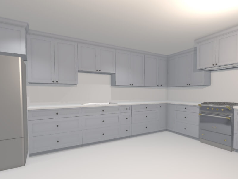
Back in November 2024, I shared a post on X about a tool I was building to help visualize kitchen remodels. The response from the Three.js community was overwhelmingly positive. The demo showed how procedural rendering techniques—often used in games—can be applied to real-world use cases like designing and rendering an entire kitchen in under 60 seconds.
In this article, I’ll walk through the process and thinking behind building this kind of procedural 3D kitchen design tool using vanilla Three.js and TypeScript—from drawing walls and defining cabinet segments to auto-generating full kitchen layouts. Along the way, I’ll share key technical choices, lessons learned, and ideas for where this could evolve next.
Have been wanting to redesign my parents’ kitchen for a while now
…so I built them a little 3D kitchen design-tool with @threejs, so they can quickly prototype floorplans/ideas
Here’s me designing a full kitchen remodel in ~60s 🙂
You can try out an interactive demo of the latest version here: https://kitchen-designer-demo.vercel.app/. (Tip: Press the “/” key to toggle between 2D and 3D views.)
Designing Room Layouts with Walls
Example of user drawing a simple room shape using the built-in wall module.
To initiate our project, we begin with the wall drawing module. At a high level, this is akin to Figma’s pen tool, where the user can add one line segment at a time until a closed—or open-ended—polygon is complete on an infinite 2D canvas. In our build, each line segment represents a single wall as a 2D plane from coordinate A to coordinate B, while the complete polygon outlines the perimeter envelope of a room.
We begin by capturing the [X, Z] coordinates (with Y oriented upwards) of the user’s initial click on the infinite floor plane. This 2D point is obtained via Three.js’s built-in raycaster for intersection detection, establishing Point A.
As the user hovers the cursor over a new spot on the floor, we apply the same intersection logic to determine a temporary Point B. During this movement, a preview line segment appears, connecting the fixed Point A to the dynamic Point B for visual feedback.
Upon the user’s second click to confirm Point B, we append the line segment (defined by Points A and B) to an array of segments. The former Point B instantly becomes the new Point A, allowing us to continue the drawing process with additional line segments.
Here is a simplified code snippet demonstrating a basic 2D pen-draw tool using Three.js:
import * as THREE from 'three';
const scene = new THREE.Scene();
const camera = new THREE.PerspectiveCamera(75, window.innerWidth / window.innerHeight, 0.1, 1000);
camera.position.set(0, 5, 10); // Position camera above the floor looking down
camera.lookAt(0, 0, 0);
const renderer = new THREE.WebGLRenderer();
renderer.setSize(window.innerWidth, window.innerHeight);
document.body.appendChild(renderer.domElement);
// Create an infinite floor plane for raycasting
const floorGeometry = new THREE.PlaneGeometry(100, 100);
const floorMaterial = new THREE.MeshBasicMaterial({ color: 0xcccccc, side: THREE.DoubleSide });
const floor = new THREE.Mesh(floorGeometry, floorMaterial);
floor.rotation.x = -Math.PI / 2; // Lay flat on XZ plane
scene.add(floor);
const raycaster = new THREE.Raycaster();
const mouse = new THREE.Vector2();
let points: THREE.Vector3[] = []; // i.e. wall endpoints
let tempLine: THREE.Line | null = null;
const walls: THREE.Line[] = [];
function getFloorIntersection(event: MouseEvent): THREE.Vector3 | null {
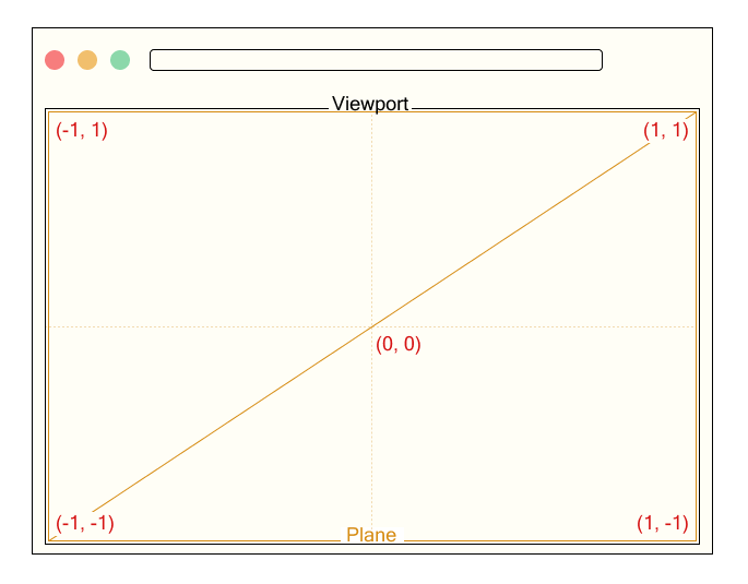
mouse.x = (event.clientX / window.innerWidth) * 2 - 1;
mouse.y = -(event.clientY / window.innerHeight) * 2 + 1;
raycaster.setFromCamera(mouse, camera);
const intersects = raycaster.intersectObject(floor);
if (intersects.length > 0) {
// Round to simplify coordinates (optional for cleaner drawing)
const point = intersects[0].point;
point.x = Math.round(point.x);
point.z = Math.round(point.z);
point.y = 0; // Ensure on floor plane
return point;
}
return null;
}
// Update temporary line preview
function onMouseMove(event: MouseEvent) {
const point = getFloorIntersection(event);
if (point && points.length > 0) {
// Remove old temp line if exists
if (tempLine) {
scene.remove(tempLine);
tempLine = null;
}
// Create new temp line from last point to current hover
const geometry = new THREE.BufferGeometry().setFromPoints([points[points.length - 1], point]);
const material = new THREE.LineBasicMaterial({ color: 0x0000ff }); // Blue for temp
tempLine = new THREE.Line(geometry, material);
scene.add(tempLine);
}
}
// Add a new point and draw permanent wall segment
function onMouseDown(event: MouseEvent) {
if (event.button !== 0) return; // Left click only
const point = getFloorIntersection(event);
if (point) {
points.push(point);
if (points.length > 1) {
// Draw permanent wall line from previous to current point
const geometry = new THREE.BufferGeometry().setFromPoints([points[points.length - 2], points[points.length - 1]]);
const material = new THREE.LineBasicMaterial({ color: 0xff0000 }); // Red for permanent
const wall = new THREE.Line(geometry, material);
scene.add(wall);
walls.push(wall);
}
// Remove temp line after click
if (tempLine) {
scene.remove(tempLine);
tempLine = null;
}
}
}
// Add event listeners
window.addEventListener('mousemove', onMouseMove);
window.addEventListener('mousedown', onMouseDown);
// Animation loop
function animate() {
requestAnimationFrame(animate);
renderer.render(scene, camera);
}
animate();
The above code snippet is a very basic 2D pen tool, and yet this information is enough to generate an entire room instance. For reference: not only does each line segment represent a wall (2D plane), but the set of accumulated points can also be used to auto-generate the room’s floor mesh, and likewise the ceiling mesh (the inverse of the floor mesh).
In order to view the planes representing the walls in 3D, one can transform each THREE.Line into a custom Wall class object, which contains both a line (for orthogonal 2D “floor plan” view) and a 2D inward-facing plane (for perspective 3D “room” view). To build this class:
class Wall extends THREE.Group {
  constructor(length: number, height: number = 96, thickness: number = 4) {
    super();

    // 2D line for top view, along the x-axis
    const lineGeometry = new THREE.BufferGeometry().setFromPoints([
      new THREE.Vector3(0, 0, 0),
      new THREE.Vector3(length, 0, 0),
    ]);
    const lineMaterial = new THREE.LineBasicMaterial({ color: 0xff0000 });
    const line = new THREE.Line(lineGeometry, lineMaterial);
    this.add(line);

    // 3D wall as a box for thickness
    const wallGeometry = new THREE.BoxGeometry(length, height, thickness);
    const wallMaterial = new THREE.MeshBasicMaterial({ color: 0xaaaaaa, side: THREE.DoubleSide });
    const wall = new THREE.Mesh(wallGeometry, wallMaterial);
    wall.position.set(length / 2, height / 2, 0);
    this.add(wall);
  }
}
We can now update the wall draw module to utilize this newly created Wall object:
// Update our variables
let tempWall: Wall | null = null;
const walls: Wall[] = [];

// Replace line creation in onMouseDown with
if (points.length > 1) {
  const start = points[points.length - 2];
  const end = points[points.length - 1];
  const direction = end.clone().sub(start);
  const length = direction.length();
  const wall = new Wall(length);
  wall.position.copy(start);
  wall.rotation.y = Math.atan2(direction.z, direction.x); // Align along direction (assuming CCW for inward facing)
  scene.add(wall);
  walls.push(wall);
}
Upon adding the floor and ceiling meshes, we can further transform our wall module into a room generation module. To recap what we have just created: by adding walls one by one, we have given the user the ability to create full rooms with walls, floors, and ceilings—all of which can be adjusted later in the scene.
User dragging out the wall in 3D perspective camera-view.
Generating Cabinets with Procedural Modeling
Our cabinet-related logic can consist of countertops, base cabinets, and wall cabinets.
Rather than taking several minutes to add the cabinets on a case-by-case basis—for example, like with IKEA’s 3D kitchen builder—it’s possible to add all the cabinets at once via a single user action. One method to employ here is to allow the user to draw high-level cabinet line segments, in the same manner as the wall draw module.
In this module, each cabinet segment will transform into a linear row of base and wall cabinets, along with a parametrically generated countertop mesh on top of the base cabinets. As the user creates the segments, we can automatically populate this line segment with pre-made 3D cabinet meshes in meshing software like Blender. Ultimately, each cabinet’s width, depth, and height parameters will be fixed, while the width of the last cabinet can be dynamic to fill the remaining space. We use a cabinet filler piece mesh here—a regular plank, with its scale-X parameter stretched or compressed as needed.
Creating the Cabinet Line Segments
User can make a half-peninsula shape by dragging the cabinetry line segments alongside the walls, then in free-space.
Here we will construct a dedicated cabinet module, with the aforementioned cabinet line segment logic. This process is very similar to the wall drawing mechanism, where users can draw straight lines on the floor plane using mouse clicks to define both start and end points. Unlike walls, which can be represented by simple thin lines, cabinet line segments need to account for a standard depth of 24 inches to represent the base cabinets’ footprint. These segments do not require closing-polygon logic, as they can be standalone rows or L-shapes, as is common in most kitchen layouts.
We can further improve the user experience by incorporating snapping functionality, where the endpoints of a cabinet line segment automatically align to nearby wall endpoints or wall intersections, if within a certain threshold (e.g., 4 inches). This ensures cabinets fit snugly against walls without requiring manual precision. For simplicity, we’ll outline the snapping logic in code but focus on the core drawing functionality.
We can start by defining the CabinetSegment class. Like the walls, this should be its own class, as we will later add the auto-populating 3D cabinet models.
class CabinetSegment extends THREE.Group {
  public length: number;

  constructor(length: number, height: number = 96, depth: number = 24, color: number = 0xff0000) {
    super();
    this.length = length;
    const geometry = new THREE.BoxGeometry(length, height, depth);
    const material = new THREE.MeshBasicMaterial({ color, wireframe: true });
    const box = new THREE.Mesh(geometry, material);
    box.position.set(length / 2, height / 2, depth / 2); // Shift so depth spans 0 to depth (inward)
    this.add(box);
  }
}
Once we have the cabinet segment, we can use it in a manner very similar to the wall line segments:
let cabinetPoints: THREE.Vector3[] = [];
let tempCabinet: CabinetSegment | null = null;
const cabinetSegments: CabinetSegment[] = [];
const CABINET_DEPTH = 24; // everything in inches
const CABINET_SEGMENT_HEIGHT = 96; // i.e. both wall & base cabinets -> group should extend to ceiling
const SNAPPING_DISTANCE = 4;

function getSnappedPoint(point: THREE.Vector3): THREE.Vector3 {
  // Simple snapping: check against existing wall points (wallPoints array from wall module)
  for (const wallPoint of wallPoints) {
    if (point.distanceTo(wallPoint) < SNAPPING_DISTANCE) return wallPoint;
  }
  return point;
}

// Update temporary cabinet preview
function onMouseMoveCabinet(event: MouseEvent) {
  const point = getFloorIntersection(event);
  if (point && cabinetPoints.length > 0) {
    const snappedPoint = getSnappedPoint(point);
    if (tempCabinet) {
      scene.remove(tempCabinet);
      tempCabinet = null;
    }
    const start = cabinetPoints[cabinetPoints.length - 1];
    const direction = snappedPoint.clone().sub(start);
    const length = direction.length();
    if (length > 0) {
      tempCabinet = new CabinetSegment(length, CABINET_SEGMENT_HEIGHT, CABINET_DEPTH, 0x0000ff); // Blue for temp
      tempCabinet.position.copy(start);
      tempCabinet.rotation.y = Math.atan2(direction.z, direction.x);
      scene.add(tempCabinet);
    }
  }
}

// Add a new point and draw permanent cabinet segment
function onMouseDownCabinet(event: MouseEvent) {
  if (event.button !== 0) return;
  const point = getFloorIntersection(event);
  if (point) {
    const snappedPoint = getSnappedPoint(point);
    cabinetPoints.push(snappedPoint);
    if (cabinetPoints.length > 1) {
      const start = cabinetPoints[cabinetPoints.length - 2];
      const end = cabinetPoints[cabinetPoints.length - 1];
      const direction = end.clone().sub(start);
      const length = direction.length();
      if (length > 0) {
        const segment = new CabinetSegment(length, CABINET_SEGMENT_HEIGHT, CABINET_DEPTH, 0xff0000); // Red for permanent
        segment.position.copy(start);
        segment.rotation.y = Math.atan2(direction.z, direction.x);
        scene.add(segment);
        cabinetSegments.push(segment);
      }
    }
    if (tempCabinet) {
      scene.remove(tempCabinet);
      tempCabinet = null;
    }
  }
}

// Add separate event listeners for cabinet mode (e.g., toggled via UI button)
window.addEventListener('mousemove', onMouseMoveCabinet);
window.addEventListener('mousedown', onMouseDownCabinet);
Auto-Populating the Line Segments with Live Cabinet Models
Here we fill 2 line-segments with 3D cabinet models (base & wall), and countertop meshes.
Once the cabinet line segments are defined, we can procedurally populate them with detailed components. This involves dividing each segment vertically into three layers: base cabinets at the bottom, countertops in the middle, and wall cabinets above. For the base and wall cabinets, we’ll use an optimization function to divide the segment’s length into standard widths (preferring 30-inch cabinets), with any remainder filled using the filler piece mentioned above. Countertops are even simpler—they form a single continuous slab stretching the full length of the segment.
The base cabinets are set to 24 inches deep and 34.5 inches high. Countertops add 1.5 inches in height and extend to 25.5 inches deep (including a 1.5-inch overhang). Wall cabinets start at 54 inches high (18 inches above the countertop), measure 12 inches deep, and are 30 inches tall. After generating these placeholder bounding boxes, we can replace them with preloaded 3D models from Blender using a loading function (e.g., via GLTFLoader).
To handle individual cabinets, we’ll create a simple Cabinet class that manages the placeholder and model loading.
import { GLTFLoader } from 'three/examples/jsm/loaders/GLTFLoader.js';

const loader = new GLTFLoader();

class Cabinet extends THREE.Group {
  constructor(width: number, height: number, depth: number, modelPath: string, color: number) {
    super();

    // Placeholder box
    const geometry = new THREE.BoxGeometry(width, height, depth);
    const material = new THREE.MeshBasicMaterial({ color });
    const placeholder = new THREE.Mesh(geometry, material);
    this.add(placeholder);


    // Load and replace with model async

    // Case: Non-standard width -> use filler piece
    if (width < DEFAULT_MODEL_WIDTH) {
      loader.load(FILLER_PIECE_FALLBACK_PATH, (gltf) => {
        const model = gltf.scene;
        model.scale.set(
          width / FILLER_PIECE_WIDTH,
          height / FILLER_PIECE_HEIGHT,
          depth / FILLER_PIECE_DEPTH,
        );
        this.add(model);
        this.remove(placeholder);
      });
    }

    loader.load(modelPath, (gltf) => {
      const model = gltf.scene;
      model.scale.set(width / DEFAULT_MODEL_WIDTH, 1, 1); // Scale width
      this.add(model);
      this.remove(placeholder);
    });
  }
}
Then, we can add a populate method to the existing CabinetSegment class:
function splitIntoCabinets(width: number): number[] {
  const cabinets = [];
  // Preferred width
  while (width >= DEFAULT_MODEL_WIDTH) {
    cabinets.push(DEFAULT_MODEL_WIDTH);
    width -= DEFAULT_MODEL_WIDTH;
  }
  if (width > 0) {
    cabinets.push(width); // Custom empty slot
  }
  return cabinets;
}

class CabinetSegment extends THREE.Group {
  // ... (existing constructor and properties)

  populate() {
    // Remove placeholder line and box
    while (this.children.length > 0) {
      this.remove(this.children[0]);
    }

    let offset = 0;
    const widths = splitIntoCabinets(this.length);

    // Base cabinets
    widths.forEach((width) => {
      const baseCab = new Cabinet(width, BASE_HEIGHT, BASE_DEPTH, 'models/base_cabinet.glb', 0x8b4513);
      baseCab.position.set(offset + width / 2, BASE_HEIGHT / 2, BASE_DEPTH / 2);
      this.add(baseCab);
      offset += width;
    });

    // Countertop (single slab, no model)
    const counterGeometry = new THREE.BoxGeometry(this.length, COUNTER_HEIGHT, COUNTER_DEPTH);
    const counterMaterial = new THREE.MeshBasicMaterial({ color: 0xa9a9a9 });
    const counter = new THREE.Mesh(counterGeometry, counterMaterial);
    counter.position.set(this.length / 2, BASE_HEIGHT + COUNTER_HEIGHT / 2, COUNTER_DEPTH / 2);
    this.add(counter);

    // Wall cabinets
    offset = 0;
    widths.forEach((width) => {
      const wallCab = new Cabinet(width, WALL_HEIGHT, WALL_DEPTH, 'models/wall_cabinet.glb', 0x4b0082);
      wallCab.position.set(offset + width / 2, WALL_START_Y + WALL_HEIGHT / 2, WALL_DEPTH / 2);
      this.add(wallCab);
      offset += width;
    });
  }
}

// Call for each cabinetSegment after drawing
cabinetSegments.forEach((segment) => segment.populate());
Further Improvements & Optimizations
We can further improve the scene with appliances, varying-height cabinets, crown molding, etc.
At this point, we should have the foundational elements of room and cabinet creation logic fully in place. In order to take this project from a rudimentary segment-drawing app into the practical realm—along with dynamic cabinets, multiple realistic material options, and varying real appliance meshes—we can further enhance the user experience through several targeted refinements:
We can implement a detection mechanism to determine if a cabinet line segment is in contact with a wall line segment.
For cabinet rows that run parallel to walls, we can automatically incorporate a backsplash in the space between the wall cabinets and the countertop surface.
For cabinet segments not adjacent to walls, we can remove the upper wall cabinets and extend the countertop by an additional 15 inches, aligning with standard practices for kitchen islands or peninsulas.
We can introduce drag-and-drop functionality for appliances, each with predefined widths, allowing users to position them along the line segment. This integration will instruct our cabinet-splitting algorithm to exclude those areas from dynamic cabinet generation.
Additionally, we can give users more flexibility by enabling the swapping of one appliance with another, applying different textures to our 3D models, and adjusting default dimensions—such as wall cabinet depth or countertop overhang—to suit specific preferences.
All these core components lead us to a comprehensive, interactive application that enables the rapid rendering of a complete kitchen: cabinets, countertops, and appliances, in a fully interactive, user-driven experience.
The aim of this project is to demonstrate that complex 3D tasks can be distilled down to simple user actions. It is fully possible to take the high-dimensional complexity of 3D tooling—with seemingly limitless controls—and encode these complexities into low-dimensional, easily adjustable parameters. Whether the developer chooses to expose these parameters to the user or an LLM, the end result is that historically complicated 3D processes can become simple, and thus the entire contents of a 3D scene can be fully transformed with only a few parameters.
If you find this type of development interesting, have any great ideas, or would love to contribute to the evolution of this product, I strongly welcome you to reach out to me via email. I firmly believe that only recently has it become possible to build home design software that is so wickedly fast and intuitive that any person—regardless of architectural merit—will be able to design their own single-family home in less than 5 minutes via a web app, while fully adhering to local zoning, architectural, and design requirements. All the infrastructure necessary to accomplish this already exists; all it takes is a team of crazy, ambitious developers looking to change the standard of architectural home design.
When Flash was taken from us all those years ago, it felt like losing a creative home — suddenly, there were no tools left for building truly interactive experiences on the web. In its place, the web flattened into a static world of HTML and CSS.
But those days are finally behind us. We’re picking up where we left off nearly two decades ago, and the web is alive again with rich, immersive experiences — thanks in large part to powerful tools like Three.js.
I’ve been working with images, video, and interactive projects for 15 years, using things like Processing, p5.js, OpenFrameworks, and TouchDesigner. Last year, I added Three.js to the mix as a creative tool, and I’ve been loving the learning process. That ongoing exploration leads to little experiments like the one I’m sharing in this tutorial.
Project Structure
The structure of our script is going to be simple: one function to preload assets, and another one to build the scene.
Since we’ll be working with 3D text, the first thing we need to do is load a font in .json format — the kind that works with Three.js.
To convert a .ttf font into that format, you can use the Facetype.js tool, which generates a .typeface.json file.
const Resources = {
	font: null
};

function preload() {

	const _font_loader = new FontLoader();
	_font_loader.load( "../static/font/Times New Roman_Regular.json", ( font ) => {

		Resources.font = font;
		init();

	} );

}

function init() {

}

window.onload = preload;
Scene setup & Environment
A classic Three.js scene — the only thing to keep in mind is that we’re working with Three Shader Language (TSL), which means our renderer needs to be a WebGPURenderer.
const scene = new THREE.Scene();
const camera = new THREE.PerspectiveCamera(75, window.innerWidth / window.innerHeight, 0.1, 1000);
const renderer = new THREE.WebGPURenderer({ antialias: true });

document.body.appendChild(renderer.domElement);

renderer.setSize(window.innerWidth, window.innerHeight);
camera.position.z = 5;

scene.add(camera);
Next, we’ll set up the scene environment to get some lighting going.
To keep things simple and avoid loading more assets, we’ll use the default RoomEnvironment that “comes” with Three.js. We’ll also add a DirectionalLight to the scene.
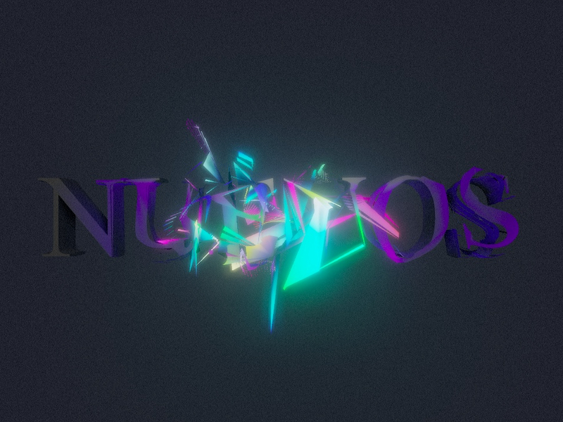
By default, the origin of the text sits at (0, 0), but we want it centered. To do that, we need to compute its BoundingBox and manually apply a translation to the geometry:
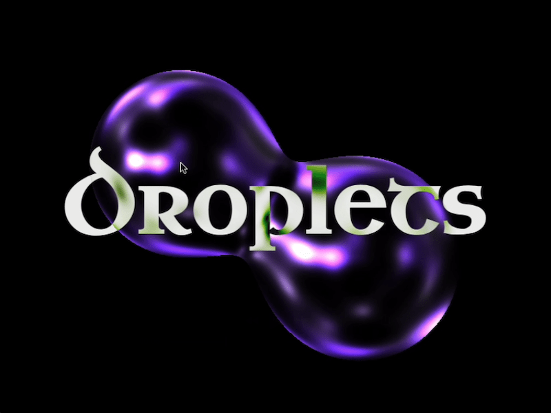
Now that we have the mesh and material ready, we can move on to the function that lets us blow everything up 💥
Three Shader Language
I really love TSL — it’s closed the gap between ideas and execution, in a context that’s not always the friendliest… shaders.
The effect we’re going to implement deforms the geometry’s vertices based on the pointer’s position, and uses spring physics to animate those deformations in a dynamic way.
But before we get to that, let’s grab a few attributes we’ll need to make everything work properly:
//  Original position of each vertex — we’ll use it as a reference
//  so unaffected vertices can "return" to their original spot
const initial_position = storage( text_geo.attributes.position, "vec3", count );

//  Normal of each vertex — we’ll use this to know which direction to "push" in
const normal_at = storage( text_geo.attributes.normal, "vec3", count );

//  Number of vertices in the geometry
const count = text_geo.attributes.position.count;
Next, we’ll create a storage buffer to hold the simulation data — and we’ll also write a function. But not a regular JavaScript function — this one’s a compute function, written in the context of TSL.
It runs on the GPU and we’ll use it to set up the initial values for our buffers, getting everything ready for the simulation.
// In this buffer we’ll store the modified positions of each vertex —
// in other words, their current state in the simulation.
const   position_storage_at = storage(new THREE.StorageBufferAttribute(count,3),"vec3",count);

const compute_init = Fn( ()=>{

	position_storage_at.element( instanceIndex ).assign( initial_position.element( instanceIndex ) );

} )().compute( count );

// Run the function on the GPU. This runs compute_init once per vertex.
renderer.computeAsync( compute_init );
Now we’re going to create another one of these functions — but unlike the previous one, this one will run inside the animation loop, since it’s responsible for updating the simulation on every frame.
This function runs on the GPU and needs to receive values from the outside — like the pointer position, for example.
To send that kind of data to the GPU, we use what’s called uniforms. They work like bridges between our “regular” code and the code that runs inside the GPU shader.
With this, we can calculate the distance between the pointer position and each vertex of the geometry.
Then we clamp that value so the deformation only affects vertices within a certain radius. To do that, we use the step function — it acts like a threshold, and lets us apply the effect only when the distance is below a defined value.
Finally, we use the vertex normal as a direction to push it outward.
const compute_update = Fn(() => {

    // Original position of the vertex — also its resting position
    const base_position = initial_position.element(instanceIndex);

    // The vertex normal tells us which direction to push
    const normal = normal_at.element(instanceIndex);

    // Current position of the vertex — we’ll update this every frame
    const current_position = position_storage_at.element(instanceIndex);

    // Calculate distance between the pointer and the base position of the vertex
    const distance = length(u_input_pos.sub(base_position));

    // Limit the effect's range: it only applies if distance is less than 0.5
    const pointer_influence = step(distance, 0.5).mul(1.0);

    // Compute the new displaced position along the normal.
    // Where pointer_influence is 0, there’ll be no deformation.
    const disorted_pos = base_position.add(normal.mul(pointer_influence));

    // Assign the new position to update the vertex
    current_position.assign(disorted_pos);

})().compute(count);
To make this work, we’re missing two key steps: we need to assign the buffer with the modified positions to the material, and we need to make sure the renderer runs the compute function on every frame inside the animation loop.
// Assign the buffer with the modified positions to the material
mesh.material.positionNode = position_storage_at.toAttribute();

// Animation loop
function animate() {
	// Run the compute function
	renderer.computeAsync(compute_update_0);

	// Render the scene
	renderer.renderAsync(scene, camera);
}
Right now the function doesn’t produce anything too exciting — the geometry moves around in a kinda clunky way. We’re about to bring in springs, and things will get much better.
// Spring — how much force we apply to reach the target value
velocity += (target_value - current_value) * spring;

// Friction controls the damping, so the movement doesn’t oscillate endlessly
velocity *= friction;

current_value += velocity;
But before that, we need to store one more value per vertex, the velocity, so let’s create another storage buffer.
const position_storage_at = storage(new THREE.StorageBufferAttribute(count, 3), "vec3", count);

// New buffer for velocity
const velocity_storage_at = storage(new THREE.StorageBufferAttribute(count, 3), "vec3", count);

const compute_init = Fn(() => {

    position_storage_at.element(instanceIndex).assign(initial_position.element(instanceIndex));

    // We initialize it too
    velocity_storage_at.element(instanceIndex).assign(vec3(0.0, 0.0, 0.0));

})().compute(count);
Now we’ve got everything we need — time to start fine-tuning.
We’re going to add two things. First, we’ll use the TSL function mx_noise_vec3 to generate some noise for each vertex. That way, we can tweak the direction a bit so things don’t feel so stiff.
We’re also going to rotate the vertices using another TSL function — surprise, it’s called rotate.
Here’s what our updated compute_update function looks like:
const compute_update = Fn(() => {

    const base_position = initial_position.element(instanceIndex);
    const current_position = position_storage_at.element(instanceIndex);
    const current_velocity = velocity_storage_at.element(instanceIndex);

    const normal = normal_at.element(instanceIndex);

    // NEW: Add noise so the direction in which the vertices "explode" isn’t too perfectly aligned with the normal
    const noise = mx_noise_vec3(current_position.mul(0.5).add(vec3(0.0, time, 0.0)), 1.0).mul(u_noise_amp);

    const distance = length(u_input_pos.sub(base_position));
    const pointer_influence = step(distance, 0.5).mul(1.5);

    const disorted_pos = base_position.add(noise.mul(normal.mul(pointer_influence)));

    // NEW: Rotate the vertices to give the animation a more chaotic feel
    disorted_pos.assign(rotate(disorted_pos, vec3(normal.mul(distance)).mul(pointer_influence)));

    disorted_pos.assign(mix(base_position, disorted_pos, u_input_pos_press));

    current_velocity.addAssign(disorted_pos.sub(current_position).mul(u_spring));
    current_position.addAssign(current_velocity);
    current_velocity.assign(current_velocity.mul(u_friction));

})().compute(count);
Now that the motion feels right, it’s time to tweak the material colors a bit and add some post-processing to the scene.
We’re going to work on the emissive color — meaning it won’t be affected by lights, and it’ll always look bright and explosive. Especially once we throw some bloom on top. (Yes, bloom everything.)
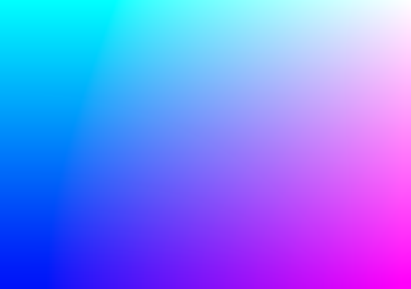
We’ll start from a base color (whichever you like), passed in as a uniform. To make sure each vertex gets a slightly different color, we’ll offset its hue a bit using values from the buffers — in this case, the velocity buffer.
The hue function takes a color and a value to shift its hue, kind of like how offsetHSL works in THREE.Color.
// Base emissive color
const emissive_color = color(new THREE.Color("0000ff"));

const vel_at = velocity_storage_at.toAttribute();
const hue_rotated = vel_at.mul(Math.PI*10.0);

// Multiply by the length of the velocity buffer — this means the more movement,
// the more the vertex color will shift
const emission_factor = length(vel_at).mul(10.0);

// Assign the color to the emissive node and boost it as much as you want
mesh.material.emissiveNode = hue(emissive_color, hue_rotated).mul(emission_factor).mul(5.0);
Finally! Lets change scene background color and add Fog:
scene.fog = new THREE.Fog(new THREE.Color("#41444c"),0.0,8.5);
scene.background = scene.fog.color;
Now, let’s spice up the scene with a bit of post-processing — one of those things that got way easier to implement thanks to TSL.
We’re going to include three effects: ambient occlusion, bloom, and noise. I always like adding some noise to what I do — it helps break up the flatness of the pixels a bit.
I won’t go too deep into this part — I grabbed the AO setup from the Three.js examples.
When building the basement studio site, we wanted to add 3D characters without compromising performance. We used instancing to render all the characters simultaneously. This post introduces instances and how to use them with React Three Fiber.
Introduction
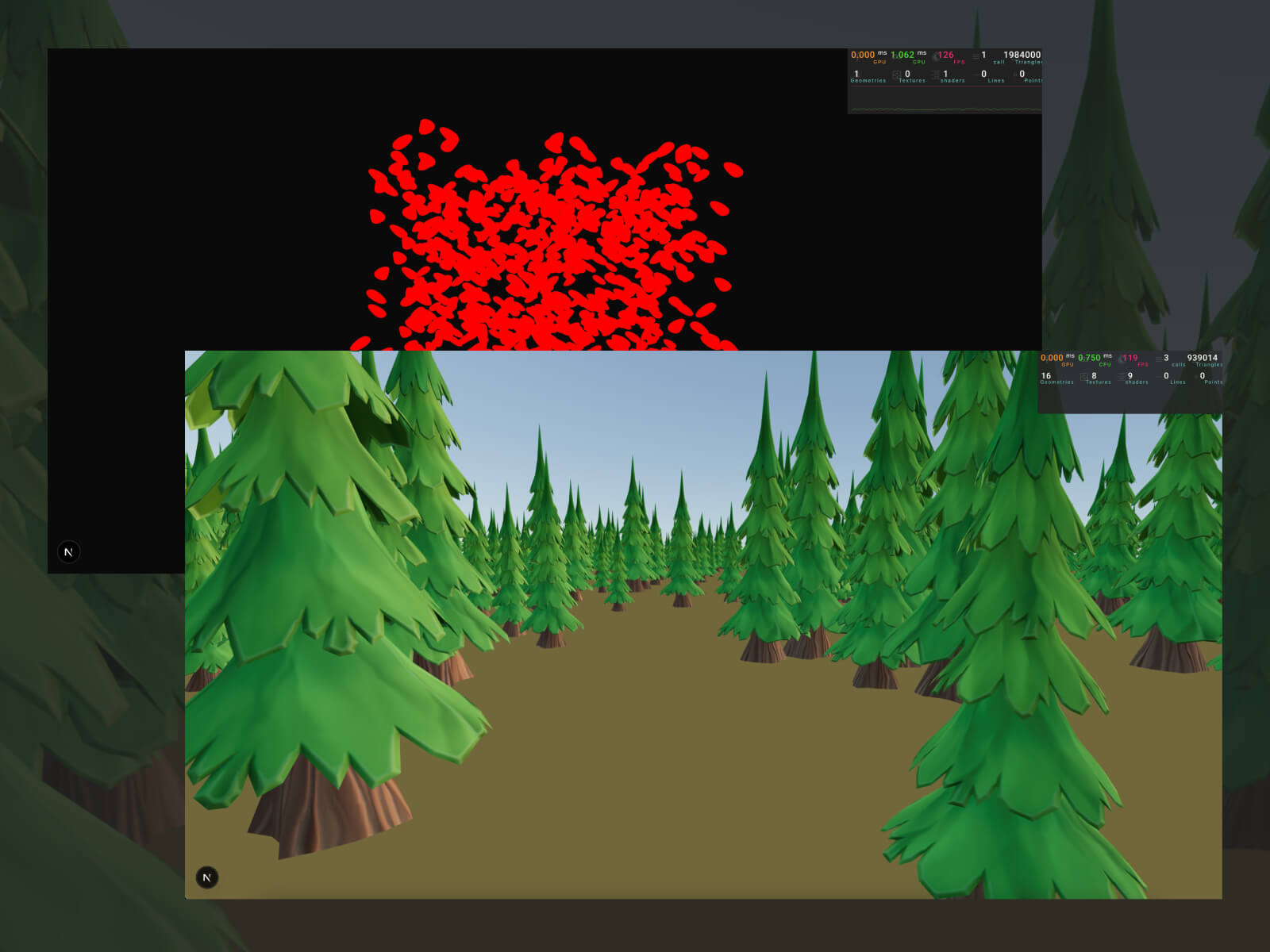
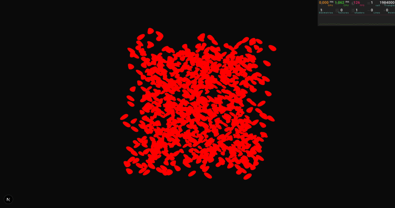
Instancing is a performance optimization that lets you render many objects that share the same geometry and material simultaneously. If you have to render a forest, you’d need tons of trees, rocks, and grass. If they share the same base mesh and material, you can render all of them in a single draw call.
A draw call is a command from the CPU to the GPU to draw something, like a mesh. Each unique geometry or material usually needs its own call. Too many draw calls hurt performance. Instancing reduces that by batching many copies into one.
Basic instancing
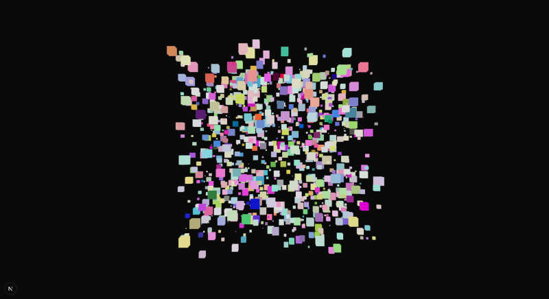
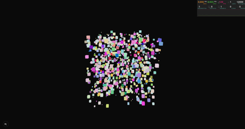
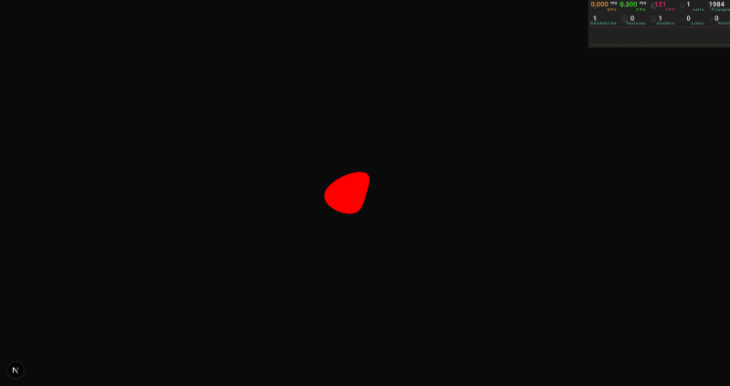
As an example, let’s start by rendering a thousand boxes in a traditional way, and let’s loop over an array and generate some random boxes:
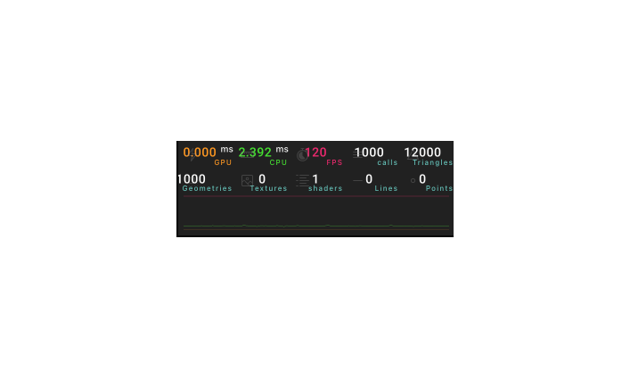
If we add a performance monitor to it, we’ll notice that the number of “calls” matches our boxCount.
A quick way to implement instances in our project is to use drei/instances.
The Instances component acts as a provider; it needs a geometry and materials as children that will be used each time we add an instance to our scene.
The Instance component will place one of those instances in a particular position/rotation/scale. Every Instance will be rendered simultaneously, using the geometry and material configured on the provider.
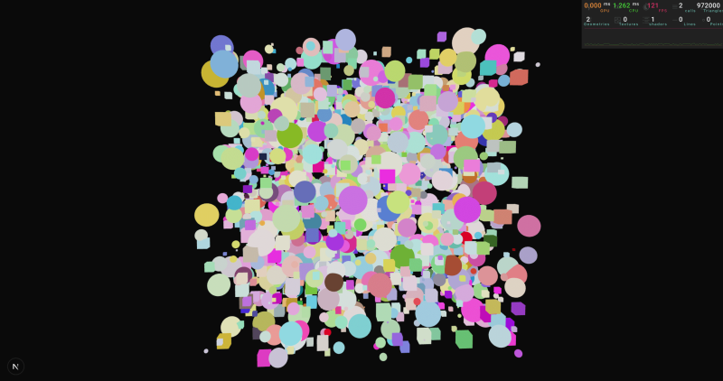
What is happening here? We are sending the geometry of our box and the material just once to the GPU, and ordering that it should reuse the same data a thousand times, so all boxes are drawn simultaneously.
Notice that we can have multiple colors even though they use the same material because Three.js supports this. However, other properties, like the map, should be the same because all instances share the exact same material.
We’ll see how we can hack Three.js to support multiple maps later in the article.
Having multiple sets of instances
If we are rendering a forest, we may need different instances, one for trees, another for rocks, and one for grass. However, the example from before only supports one instance in its provider. How can we handle that?
The creteInstnace() function from drei allows us to create multiple instances. It returns two React components, the first one a provider that will set up our instance, the second, a component that we can use to position one instance in our scene.
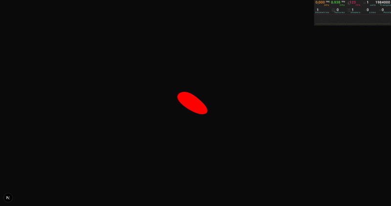
Until now, all the examples have used Three.js’ built-in materials to add our meshes to the scene, but sometimes we need to create our own materials. How can we add support for instances to our shaders?
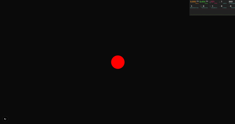
The code runs successfully, but all spheres are in the same place, even though we added different positions.
This is happening because when we calculated the position of each vertex in the vertexShader, we returned the same position for all vertices, all these attributes are the same for all spheres, so they end up in the same spot:
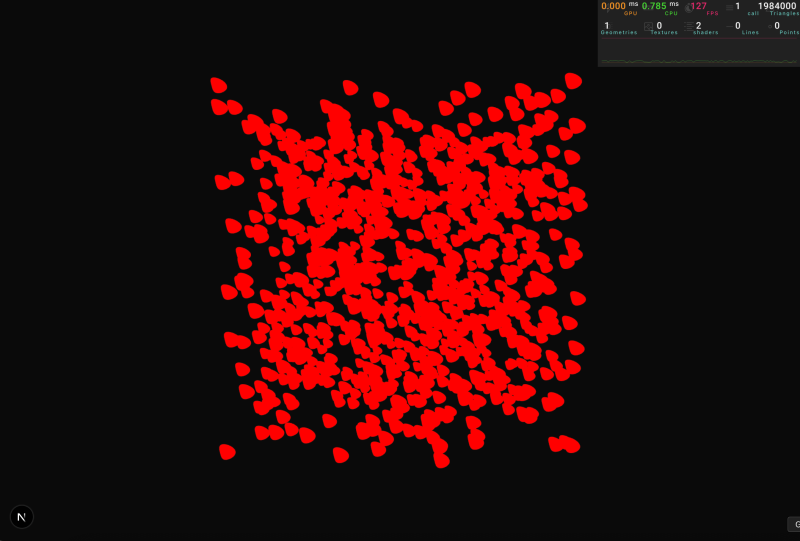
We managed to render all the blobs in different positions, but since the uniforms are shared across all instances, they all end up having the same animation.
To solve this issue, we need a way to provide custom information for each instance. We actually did this before, when we used the instanceMatrix to move each instance to its corresponding location. Let’s debug the magic behind instanceMatrix, so we can learn how we can create own instanced attributes.
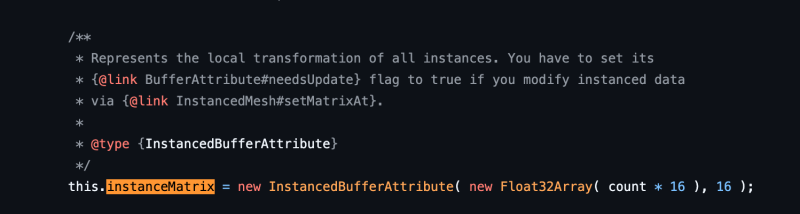
Taking a look at the implementation of instancedMatrix we can see that it is using something called InstancedAttribute:
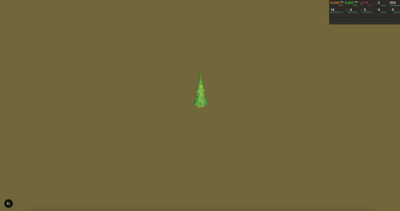
import { useGLTF } from "@react-three/drei"
import * as THREE from "three"
import { GLTF } from "three/examples/jsm/Addons.js"

// I always like to type the models so that they are safer to work with
interface TreeGltf extends GLTF {
  nodes: {
    tree_low001_StylizedTree_0: THREE.Mesh<
      THREE.BufferGeometry,
      THREE.MeshStandardMaterial
    >
  }
}

function Scene() {

  // Load the model
  const { nodes } = useGLTF(
    "/stylized_pine_tree_tree.glb"
  ) as unknown as TreeGltf

  return (
    <group>
      {/* add one tree to our scene */ }
      <mesh
        scale={0.02}
        geometry={nodes.tree_low001_StylizedTree_0.geometry}
        material={nodes.tree_low001_StylizedTree_0.material}
      />
    </group>
  )
}
(I added lights and a ground in a separate file.)
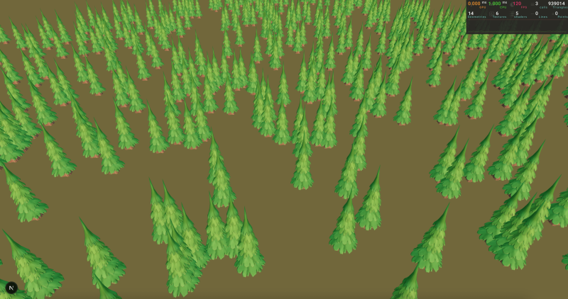
Now that we have one tree, let’s apply instancing.
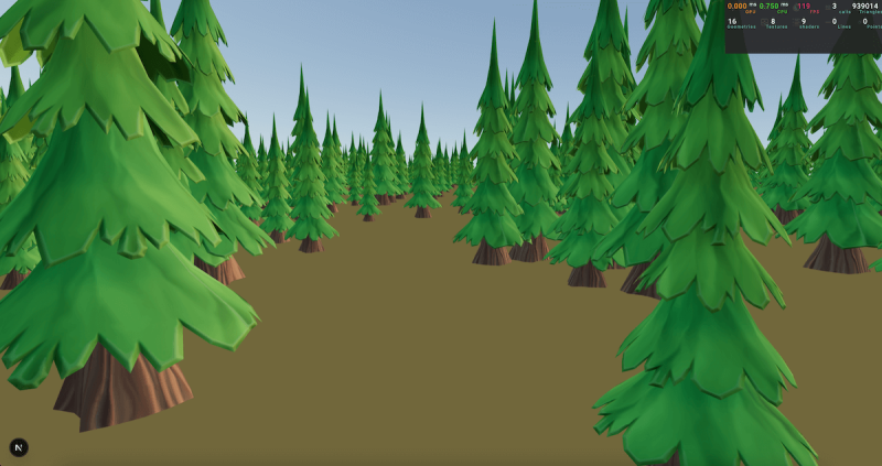
Our entire forest is being rendered in only three draw calls: one for the skybox, another one for the ground plane, and a third one with all the trees.
To make things more interesting, we can vary the height and rotation of each tree:
There are some topics that I didn’t cover in this article, but I think they are worth mentioning:
Batched Meshes: Now, we can render one geometry multiple times, but using a batched mesh will allow you to render different geometries at the same time, sharing the same material. This way, you are not limited to rendering one tree geometry; you can vary the shape of each one.
Skeletons: They are not currently supported with instancing, to create the latest basement.studio site we managed to hack our own implementation, I invite you to read our implementation there.
Morphing with batched mesh: Morphing is supported with instances but not with batched meshes. If you want to implement it yourself, I’d suggest you read these notes.
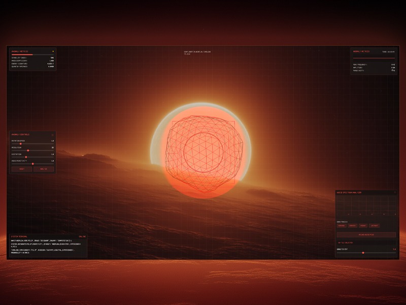
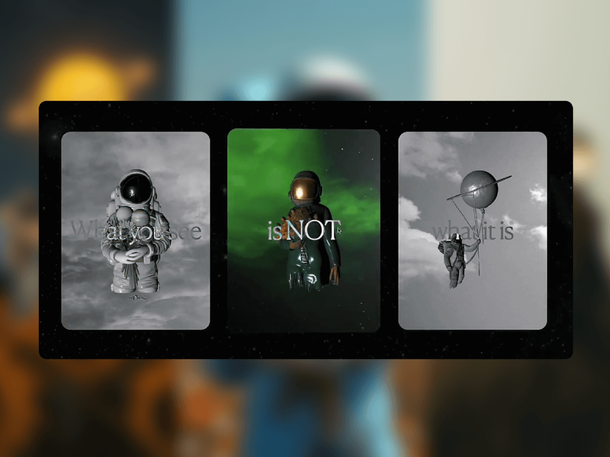
Sound is vibration, vision is vibration you can see. I’m always chasing the moment those waves overlap. For a recent Webflow & GSAP community challenge focusing on GSAP Draggable and Inertia Plugin, I decided to push the idea further by building a futuristic audio-reactive visualizer. The concept was to create a sci-fi “anomaly detector” interface that reacts to music in real time, blending moody visuals with sound.
The concept began with a simple image in my mind: a glowing orange-to-white sphere sitting alone in a dark void, the core that would later pulse with the music. To solidify the idea, I ran this prompt through Midjourney: “Glowing orange and white gradient sphere, soft blurry layers, smooth distortion, dark black background, subtle film-grain, retro-analog vibe, cinematic lighting.” After a few iterations I picked the frame that felt right, gave it a quick color pass in Photoshop, and used that clean, luminous orb as the visual foundation for the entire audio-reactive build.
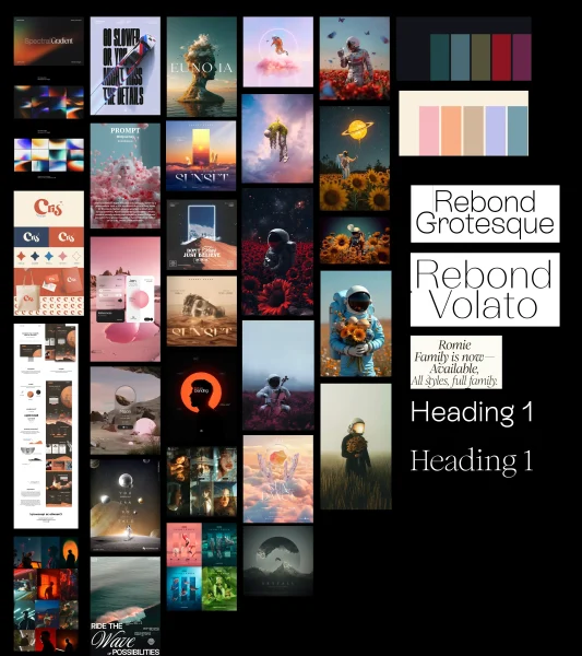
Midjourney explorations
The project was originally built as an entry for the Webflow × GSAP Community Challenge (Week 2: “Draggable & Inertia”), which encouraged the use of GSAP’s dragging and inertia capabilities. This context influenced the features: I made the on-screen control panels draggable with momentum, and even gave the 3D orb a subtle inertia-driven movement when “flung”. In this article, I’ll walk you through the entire process – from setting up the Three.js scene and analyzing audio with the Web Audio API, to creating custom shaders and adding GSAP animations and interactivity. By the end, you’ll see how code, visuals, and sound come together to create an immersive audio visualizer.
Setting Up the Three.js Scene
To build the 3D portion, I used Three.js to create a scene containing a dynamic sphere (the “anomaly”) and other visual elements.
We start with the usual Three.js setup: a scene, a camera, and a renderer. I went with a perspective camera to get a nice 3D view of our orb and placed it a bit back so the object is fully in frame.
An OrbitControls is used to allow basic click-and-drag orbiting around the object (with some damping for smoothness). Here’s a simplified snippet of the initial setup:
// Initialize Three.js scene, camera, renderer
const scene = new THREE.Scene();
const camera = new THREE.PerspectiveCamera(75, window.innerWidth/window.innerHeight, 0.1, 100);
camera.position.set(0, 0, 10);  // camera back a bit from origin

const renderer = new THREE.WebGLRenderer({ antialias: true });
renderer.setSize(window.innerWidth, window.innerHeight);
document.body.appendChild(renderer.domElement);

// Add OrbitControls for camera rotation
const controls = new THREE.OrbitControls(camera, renderer.domElement);
controls.enableDamping = true;
controls.dampingFactor = 0.1;
controls.rotateSpeed = 0.5;
controls.enableZoom = false; // lock zoom for a more fixed view
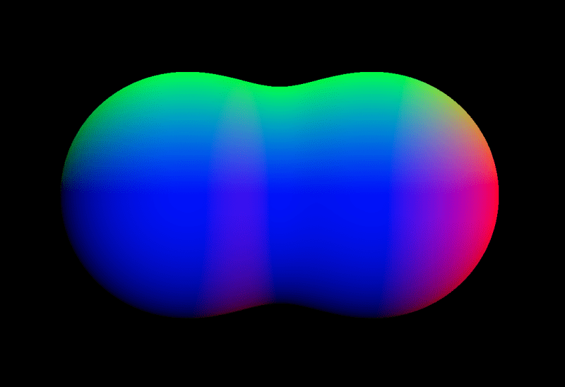
Next, I created the anomaly object. This is the main feature: a spiky wireframe sphere that reacts to audio. Three.js provides shapes like SphereGeometry or IcosahedronGeometry that we can use for a sphere. I chose an icosahedron geometry because it gives an interesting multi sided look and allows easy control of detail (via a subdivision level). The anomaly is actually composed of two overlapping parts:
Outer wireframe sphere: An IcosahedronGeometry with a custom ShaderMaterial that draws it as a glowing wireframe. This part will distort based on music (imagine it “vibrating” and morphing with the beat).
Inner glow sphere: A slightly larger SphereGeometry drawn with a semi-transparent, emissive shader (using the backside of the geometry) to create a halo or aura around the wireframe. This gives the orb a warm glow effect, like an energy field.
I also added in some extra visuals: a field of tiny particles floating in the background (for a depth effect, like dust or sparks) and a subtle grid overlay in the UI (more on the UI later). The scene’s background is set to a dark color, and I layered a background image (the edited Midjourney visual) behind the canvas to create the mysterious-alien landscape horizon. This combination of 3D objects and 2D backdrop creates the illusion of a holographic display over a planetary surface.
Integrating the Web Audio API for Music Analysis
With the 3D scene in place, the next step was making it respond to music. This is where the Web Audio API comes in. I allowed the user to either upload an audio file or pick one of the four provided tracks. When the audio plays, we tap into the audio stream and analyze its frequencies in real-time using an AnalyserNode. The AnalyserNode gives us access to frequency data. This is a snapshot of the audio spectrum (bass, mids, treble levels, etc.) at any given moment, which we can use to drive animations.
To set this up, I created an AudioContext and an AnalyserNode, and connected an audio source to it. If you’re using an <audio> element for playback, you can create a MediaElementSource from it and pipe that into the analyser. For example:
// Create AudioContext and Analyser
const audioContext = new (window.AudioContext || window.webkitAudioContext)();
const analyser = audioContext.createAnalyser();
analyser.fftSize = 2048;                  // Use an FFT size of 2048 for analysis
analyser.smoothingTimeConstant = 0.8;     // Smooth out the frequencies a bit

// Connect an audio element source to the analyser
const audioElement = document.getElementById('audio-player');  // <audio> element
const source = audioContext.createMediaElementSource(audioElement);
source.connect(analyser);
analyser.connect(audioContext.destination);  // connect to output so sound plays
Here we set fftSize to 2048, which means the analyser will break the audio into 1024 frequency bins (frequencyBinCount is half of fftSize). We also set a smoothingTimeConstant to make the data less jumpy frame-to-frame. Now, as the audio plays, we can repeatedly query the analyser for data. The method analyser.getByteFrequencyData(array) fills an array with the current frequency magnitudes (0–255) across the spectrum. Similarly, getByteTimeDomainData gives waveform amplitude data. In our animation loop, I call analyser.getByteFrequencyData() on each frame to get fresh data:
const frequencyData = new Uint8Array(analyser.frequencyBinCount);

function animate() {
  requestAnimationFrame(animate);

  // ... update Three.js controls, etc.
  if (analyser) {
    analyser.getByteFrequencyData(frequencyData);
    // Compute an average volume level from frequency data
    let sum = 0;
    for (let i = 0; i < frequencyData.length; i++) {
      sum += frequencyData[i];
    }
    const average = sum / frequencyData.length;
    let audioLevel = average / 255;  // normalize to 0.0–1.0
    // Apply a sensitivity scaling (from a UI slider)
    audioLevel *= (sensitivity / 5.0);
    // Now audioLevel represents the intensity of the music (0 = silence, ~1 = very loud)
  }

  // ... (use audioLevel to update visuals)
  renderer.render(scene, camera);
}
In my case, I also identified a “peak frequency” (the frequency bin with the highest amplitude at a given moment) and some other metrics just for fun, which I display on the UI (e.g. showing the dominant frequency in Hz, amplitude, etc., as “Anomaly Metrics”). But the key takeaway is the audioLevel – a value representing overall music intensity – which we’ll use to drive the 3D visual changes.
Syncing Audio with Visuals: Once we have audioLevel, we can inject it into our Three.js world. I passed this value into the shaders as a uniform every frame, and also used it to tweak some high-level motion (like rotation speed). Additionally, GSAP animations were triggered by play/pause events (for example, a slight camera zoom when music starts, which we’ll cover next). The result is that the visuals move in time with the music:louder or more intense moments in the audio make the anomaly glow brighter and distort more, while quiet moments cause it to settle down.
Creating the Audio-Reactive Shaders
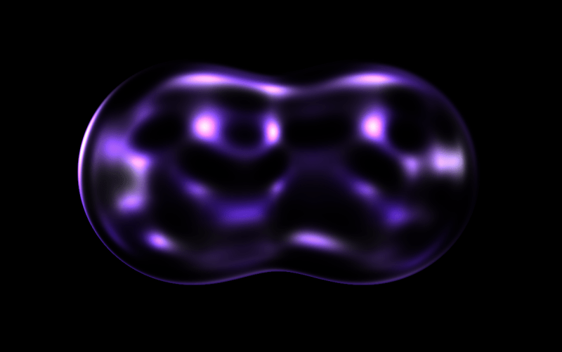
To achieve the dynamic look for the anomaly, I used custom GLSL shaders in the material. Three.js lets us write our own shaders via THREE.ShaderMaterial, which is perfect for this because it gives fine-grained control over vertex positions and fragment colors. This might sound difficult if you’re new to shaders, but conceptually we did two major things in the shader:
Vertex Distortion with Noise: We displace the vertices of the sphere mesh over time to make it wobble and spike. I included a 3D noise function (Simplex noise) in the vertex shader – it produces a smooth pseudo-random value for any 3D coordinate. For each vertex, I calculate a noise value based on its position (plus a time factor to animate it). Then I move the vertex along its normal by an amount proportional to that noise. We also multiply this by our audioLevel and a user-controlled distortion factor. Essentially, when the music is intense (high audioLevel), the sphere gets spikier and more chaotic; when the music is soft or paused, the sphere is almost smooth.
Fresnel Glow in Fragment Shader: To make the wireframe edges glow and fade realistically, I used a fresnel effect in the fragment shader. This effect makes surfaces more luminous at glancing angles. We calculate it by taking the dot product of the view direction and the vertex normal – it results in a value that’s small on edges (grazing angles) and larger on faces directly facing the camera. By inverting and exponentiating this, we get a nice glow on the outline of the sphere that intensifies at the edges. I modulated the fresnel intensity with the audioLevel as well, so the glow pulsates with the beat.
Let’s look at a simplified version of the shader code for the outer wireframe sphere material:
const outerMaterial = new THREE.ShaderMaterial({
  uniforms: {
    time:      { value: 0 },
    audioLevel:{ value: 0 },            // this will be updated each frame
    distortion:{ value: 1.0 },
    color:     { value: new THREE.Color(0xff4e42) }  // a reddish-orange base color
  },
  wireframe: true,
  transparent: true,
  vertexShader: `
    uniform float time;
    uniform float audioLevel;
    uniform float distortion;
    // (noise function omitted for brevity)

    void main() {
      // Start with the original position
      vec3 pos = position;
      // Calculate procedural noise value for this vertex (using its position and time)
      float noise = snoise(pos * 0.5 + vec3(0.0, 0.0, time * 0.3));
      // Displace vertex along its normal
      pos += normal * noise * distortion * (1.0 + audioLevel);
      // Standard transformation
      gl_Position = projectionMatrix * modelViewMatrix * vec4(pos, 1.0);
    }
  `,
  fragmentShader: `
    uniform vec3 color;
    uniform float audioLevel;
    varying vec3 vNormal;
    varying vec3 vPosition;

    void main() {
      // Calculate fresnel (view-angle dependent) term
      vec3 viewDir = normalize(cameraPosition - vPosition);
      float fresnel = 1.0 - max(0.0, dot(viewDir, vNormal));
      fresnel = pow(fresnel, 2.0 + audioLevel * 2.0);
      // Make the fragment color brighter on edges (fresnel) and pulse it slightly with time
      float pulse = 0.8 + 0.2 * sin(time * 2.0);
      vec3 emissiveColor = color * fresnel * pulse * (1.0 + audioLevel * 0.8);
      // Alpha fade out a bit when audio is high (to make spikes more ethereal)
      float alpha = fresnel * (0.7 - audioLevel * 0.3);
      gl_FragColor = vec4(emissiveColor, alpha);
    }
  `
});
In this shader, snoise is a Simplex noise function (not shown above) producing values ~-1 to 1. The vertex shader uses it to offset each vertex (pos += normal * noise * …). We multiply the noise by (1.0 + audioLevel) so that when audioLevel rises, the displacement increases. The distortion uniform is controlled by a slider in the UI, so the user can manually dial the overall spikiness. The fragment shader calculates a fresnel factor to make the wireframe edges glow. Notice how audioLevel factors into the power and into the final color intensity – louder audio makes the fresnel exponent higher (sharper glow) and also increases brightness a bit. We also included a gentle pulsing (sin(time)) independent of audio, just to give a constant breathing motion.
For the inner glow sphere, we used a separate ShaderMaterial: it’s basically a sphere drawn with side: THREE.BackSide (so we see the inner surface) and Additive Blending to give a blooming halo. Its fragment shader also uses a fresnel term, but with a much lower alpha so it appears as a soft haze around the orb. The inner sphere’s size is slightly larger (I used about 1.2× the radius of the outer sphere) so that the glow extends beyond the wireframe. When combined, the outer and inner shaders create the effect of a translucent, energy-filled orb whose surface ripples with music.
To tie it all together, every frame in the render loop I update the shader uniforms with the current time and audio level:
// in the animation loop:
outerMaterial.uniforms.time.value = elapsedTime;
outerMaterial.uniforms.audioLevel.value = audioLevel;
outerMaterial.uniforms.distortion.value = currentDistortion;
glowMaterial.uniforms.time.value = elapsedTime;
glowMaterial.uniforms.audioLevel.value = audioLevel;
The result is a 3D object that truly feels alive with the music, it oscillates, pulses, and glows in sync with whatever track is playing. Even the one you add.
Animations and Interactions with GSAP
With the visuals reacting to sound, I added GSAP to handle smooth animations and user interactions. GSAP is great for creating timeline sequences and tweening properties with easing, and it also comes with plugins that were perfect for this project: Draggable for click-and-drag UI, and InertiaPlugin for momentum. Best of all, every GSAP plugin is now completely free to use. Below are the key ways I used GSAP in the project:
Intro Animation & Camera Movement: When the user selects a track and hits play, I trigger a brief “activation” sequence. This involves some text appearing in the “terminal” and a slight camera zoom-in toward the orb to signal that the system is online. The camera movement was done with a simple GSAP tween of the camera’s position. For example, I defined a default camera position and a slightly closer “zoomed” position. On play, I use gsap.to() to interpolate the camera position to the zoomed-in coordinates, and on pause/stop I tween it back out. GSAP makes this kind of 3D property animation straightforward:
const defaultCameraPos = { x: 0, y: 0, z: 10 };
const zoomedCameraPos = { x: 0, y: 0, z: 7 }; // move camera closer on zoom

function zoomCameraForAudio(zoomIn) {
  const target = zoomIn ? zoomedCameraPos : defaultCameraPos;
  gsap.to(camera.position, {
    x: target.x,
    y: target.y,
    z: target.z,
    duration: 1.5,
    ease: "power2.inOut"
  });
}

// When audio starts:
zoomCameraForAudio(true);
// When audio ends or is stopped:
zoomCameraForAudio(false);
This smooth zoom adds drama when the music kicks in, drawing the viewer into the scene. The power2.inOut easing gives it a nice gentle start and stop. I also used GSAP timelines for any other scripted sequences (like fading out the “Analyzing…” overlay text after a few seconds, etc.), since GSAP’s timeline control is very handy for orchestrating arranging multiple animations in order.
Draggable UI Panels: The interface has a few UI components overlaying the 3D canvas – e.g. an “Anomaly Controls” panel (with sliders for rotation speed, distortion amount, etc.), an “Audio Spectrum Analyzer” panel (showing a bar graph of frequencies and track selection buttons), and a “System Terminal” readout (displaying log messages like a console). To make the experience playful, I made these panels draggable. Using GSAP’s Draggable plugin, I simply turned each .panel element into a draggable object:
Draggable.create(".panel", {
  type: "x,y",
  bounds: "body",         // confine dragging within the viewport
  inertia: true,          // enable momentum after release
  edgeResistance: 0.65,   // a bit of resistance at the edges
  onDragStart: () => { /* bring panel to front, etc. */ },
  onDragEnd: function() {
    // Optionally, log the velocity or other info for fun
    console.log("Panel thrown with velocity:", this.getVelocity());
  }
});
Setting inertia: true means when the user releases a panel, it will continue moving in the direction they tossed it, gradually slowing to a stop (thanks to InertiaPlugin). This little touch makes the UI feel more tactile and real – you can flick the panels around and they slide with some “weight.” According to GSAP’s docs, Draggable will automatically handle the physics when inertia is enabled , so it was plug-and-play. I also constrained dragging within the body bounds so panels don’t get lost off-screen. Each panel has a clickable header (a drag handle area), set via the handle option, to restrict where a user can grab it. Under the hood, InertiaPlugin calculates the velocity of the drag and creates a tween that smoothly decelerates the element after you let go, mimicking friction.
Interactive Orb Drag (Bonus): As a creative experiment, I even made the 3D anomaly orb itself draggable. This was a bit more involved since it’s not a DOM element, but I implemented it by raycasting for clicks on the 3D object and then rotating the object based on mouse movement. I applied a similar inertia effect manually: when you “throw” the orb, it keeps spinning and slowly comes to rest. This wasn’t using GSAP’s Draggable directly (since that works in screen space), but I did use the InertiaPlugin concept by capturing the drag velocity and then using an inertial decay on that velocity each frame. It added a fun way to interact with the visualizer – you can nudge the orb and see it respond physically. For example, if you drag and release quickly, the orb will continue rotating with momentum. This kind of custom 3D dragging is outside the scope of a basic tutorial, but it shows how you can combine your own logic with GSAP’s physics concepts to enrich interactions.
GSAP Draggable and Inertia in action
In summary, GSAP handles all the non-audio animations: the camera moves, panel drags, and little transitions in the UI. The combination of sound-reactive shader animations (running every frame based on audio data) and event-based GSAP tweens (triggered on user actions or certain times) gives a layered result where everything feels responsive and alive.
UI and Atmosphere
Finally, a few words about the surrounding UI/atmosphere which glue the experience together. The visualizer’s style was inspired by sci-fi control panels, so I leaned into that:
Control Panels and Readouts: I built the overlay UI with HTML/CSS, keeping it minimalistic (just semi-transparent dark panels with light text and a few sliders/buttons). Key controls include rotation speed (how fast the orb spins), resolution (tessellation level of the icosahedron mesh), distortion amount, audio reactivity (scaling of audio impact), and sensitivity (which adjusts how the audio’s volume is interpreted). Changing these in real-time immediately affects the Three.js scene – for example, dragging the “Resolution” slider rebuilds the icosahedron geometry with more or fewer triangles, which is a cool way to see the orb go from coarse to finely subdivided. The “Audio Spectrum Analyzer” panel displays a classic bar graph of frequencies (drawn on a canvas using the analyser data) so you have a 2D visualization accompanying the 3D one. There’s also a console-style terminal readout that logs events (like “AUDIO ANALYSIS SYSTEM INITIALIZED” or the velocity of drags in a playful GSAP log format) to reinforce the concept of a high-tech system at work.
Design elements: To boost the sci-fi feel, I added a subtle grid overlay across the whole screen. This was done with pure CSS – a pair of repeating linear gradients forming horizontal and vertical lines (1px thin, very transparent) over a transparent background . It’s barely noticeable but gives a technical texture, especially against the glow of the orb. I also added some drifting ambient particles (tiny dots) floating slowly in the background, implemented as simple divs animated with JavaScript. They move in pseudo-random orbits.
Soundtrack: I curated three atmospheric and moody tracks, along with one of my own unreleased tracks, under my music alias LXSTNGHT. The track was produced in Ableton, and it’s unfinished. The end result is an experience where design, code, and music production collide in real time.
Bringing all these elements together, the final result is an interactive art piece: you load a track, the “Audio ARK” system comes online with a flurry of text feedback, the ambient music starts playing, and the orb begins to pulse and mutate in sync with the sound. You can tweak controls or toss around panels (or the orb itself) to explore different visuals.
The combination of Three.js (for rendering and shader effects), Web Audio API (for sound analysis), and GSAP (for polished interactions) showcases how creative coding tools can merge to produce an immersive experience that engages multiple senses.
Fragment shaders allow us to create smooth, organic visuals that are difficult to achieve with standard polygon-based rendering in WebGL. One powerful example is the metaball effect, where multiple objects blend and deform seamlessly. This can be implemented using a technique called ray marching, directly within a fragment shader.
In this tutorial, we’ll walk you through how to create droplet-like, bubble spheres using Three.js and GLSL—an effect that responds interactively to your mouse movements. But first, take a look at the demo video below to see the final result in action.
Overview
Let’s take a look at the overall structure of the demo and review the steps we’ll follow to build it.
We arrange spheres along the mouse trail to create a stretchy, elastic motion.
Let’s get started!
1. Setup
We render a single fullscreen plane that covers the entire viewport.
// Output.ts

const planeGeometry = new THREE.PlaneGeometry(2.0, 2.0);
const planeMaterial = new THREE.RawShaderMaterial({
    vertexShader: base_vert,
    fragmentShader: output_frag,
    uniforms: this.uniforms,
});
const plane = new THREE.Mesh(planeGeometry, planeMaterial);
this.scene.add(plane);
We define a uniform variable named uResolution to pass the canvas size to the shader, where Common.width and Common.height represent the width and height of the canvas in pixels. This uniform will be used to normalize coordinates based on the screen resolution.
The vertex shader receives the position attribute.
Since the xy components of position originally range from -1 to 1, we convert them to a range from 0 to 1 and output them as a texture coordinate called vTexCoord. This is passed to the fragment shader and used to calculate colors or effects based on the position on the screen.
The fragment shader receives the interpolated texture coordinate vTexCoord and the uniform variable uResolution representing the canvas size. Here, we temporarily use vTexCoord to output color for testing.
Now we’re all set to start drawing in the fragment shader! Next, let’s move on to actually rendering the spheres.
2. Ray Marching
2.1. What is Ray Marching?
As mentioned at the beginning, we will use a method called ray marching to render spheres. Ray marching proceeds in the following steps:
Define the scene
Set the camera (viewing) direction
Cast rays
Evaluate the distance from the current ray position to the nearest object in the scene.
Move the ray forward by that distance
Check for a hit
For example, let’s consider a scene with three spheres. These spheres are expressed using SDFs (Signed Distance Functions), which will be explained in detail later.
First, we determine the camera direction. Once the direction is set, we cast a ray in that direction.
Next, we evaluate the distance to all objects from the current ray position, and take the minimum of these distances.
After obtaining this distance, we move the ray forward by that amount.
We repeat this process until either the ray gets close enough to an object—closer than a small threshold—or the maximum number of steps is reached. If the distance is below the threshold, we consider it a “hit” and shade the corresponding pixel.
For example, in the figure above, a hit is detected on the 8th ray marching step.
If the maximum number of steps were set to 7, the 7th step would not have hit anything yet. But since the limit is reached, the loop ends and no hit is detected.
Therefore, nothing would be rendered at that position. If parts of an object appear to be missing in the final image, it may be due to an insufficient number of steps. However, be aware that increasing the step count will also increase the computational load.
To better understand this process, try running this demo to see how it works in practice.
2.2. Signed Distance Function
In the previous section, we briefly mentioned the SDF (Signed Distance Function). Let’s take a moment to understand what it is.
An SDF is a function that returns the distance from a point to a particular shape. The key characteristic is that it returns a positive or negative value depending on whether the point is outside or inside the shape.
For example, here is the distance function for a sphere:
Here, p is a vector representing the position relative to the origin, and s is the radius of the sphere.
This function calculates how far the point p is from the surface of a sphere centered at the origin with radius s.
If the result is positive, the point is outside the sphere.
If negative, it is inside the sphere.
If the result is zero, the point is on the surface—this is considered a hit point (in practice, we detect a hit when the distance is less than a small threshold).
In this demo, we use a sphere’s distance function, but many other shapes have their own distance functions as well.
After that, inside the map function, two spheres are defined and their distances calculated using sdSphere. The variable d is initially set to a large value and updated with the min function to keep track of the shortest distance to the surface.
Then we run a ray marching loop, which updates the ray position by computing the distance to the nearest object at each step. The loop ends either after a fixed number of iterations or when the distance becomes smaller than a threshold (dist < EPS):
for ( int i = 0; i < ITR; ++ i ) {
	dist = map(ray);
	ray += rayDirection * dist;
	if ( dist < EPS ) break ;
}
Finally, we determine the output color. We use black as the default color (background), and render a white pixel only if a hit is detected:
vec3 color = vec3(0.0);

if ( dist < EPS ) {
	color = vec3(1.0);
}
We’ve successfully rendered two overlapping spheres using ray marching!
2.4. Normals
Although we successfully rendered spheres in the previous section, the scene still looks flat and lacks depth. This is because we haven’t applied any shading or visual effects that respond to surface orientation.
While we won’t implement full shading in this demo, we’ll still compute surface normals, as they’re essential for adding surface detail and other visual effects.
At first glance, this may seem hard to understand. Put simply, this computes the gradient of the distance function, which corresponds to the normal vector.
If you’ve studied vector calculus, this might be easy to understand. For many others, though, it may seem a bit difficult.
However, for those who are interested in how it works, we’ll now walk through the explanation in more detail.
The gradient of a scalar function 𝑓(𝑥,𝑦,𝑧) is simply a vector composed of its partial derivatives. It points in the direction of the greatest rate of increase of the function:
To compute this gradient numerically, we can use the central difference method. For example:
We apply the same idea for the 𝑦 and 𝑧 components. Note: The factor 2𝜀 is omitted in the code since we normalize the result using normalize().
Next, let us consider a signed distance function 𝑓(𝑥,𝑦,𝑧), which returns the shortest distance from any point in space to the surface of an object. By definition, 𝑓(𝑥,𝑦,𝑧)=0 on the surface of the object.
Assume that 𝑓 is smooth (i.e., differentiable) in the region of interest. When the point (𝑥,𝑦,𝑧) undergoes a small displacement Δ𝒓=(Δ𝑥,Δ𝑦,Δ𝑧), the change in the function value Δ𝑓 can be approximated using the first-order Taylor expansion:
Here,∇𝑓 is the gradient vector of 𝑓, and Δ𝒓 is an arbitrary small displacement vector.
Now, since 𝑓=0 on the surface and remains constant as we move along the surface (i.e., tangentially), the function value does not change, so Δ𝑓=0. Therefore:
This means that the gradient vector is perpendicular to any tangent vector Δ𝒓 on the surface. In other words, the gradient vector ∇𝑓 points in the direction of the surface normal.
Thus, the gradient of a signed distance function gives the surface normal direction at any point on the surface.
2.5. Visualizing Normals with Color
To verify that the surface normals are being calculated correctly, we can visualize them using color.
if ( dist < EPS ) {
	vec3 normal = generateNormal(ray);
	color = normal;
}
Note that within the if block, ray refers to a point on the surface of the object. So by passing ray to generateNormal, we can obtain the surface normal at the point of intersection.
When we render the scene, you’ll notice that the surface of the sphere is shaded in red, green, and blue based on the orientation of the normal vectors. This is because we’re mapping the 𝑥, 𝑦, and 𝑧 components of the normal vector to the RGB color channels respectively.
This is a common and intuitive way to debug normal vectors visually, helping us ensure they are computed correctly.
When combining two spheres with the standard min() function, a hard edge forms where the shapes intersect, resulting in an unnatural boundary. To avoid this, we can use a blending function called smoothMin, which softens the transition by merging the distance values smoothly.
This function creates a smooth, continuous connection between shapes—producing a metaball-like effect where the forms appear to merge organically.
The parameter k controls the smoothness of the blend. A higher k value results in a sharper transition (closer to min()), while a lower k produces smoother, more gradual merging.
For more details, please refer to the following two articles:
So far, we’ve covered how to calculate normals and how to smoothly blend objects.
Next, let’s tune the surface appearance to make things feel more realistic.
In this demo, we’re aiming to create droplet-like metaballs. So how can we achieve that kind of look? The key idea here is to use noise to distort the surface.
To create the droplet-like texture, we’re using value noise. If you’re unfamiliar with these noise techniques, the following articles provide helpful explanations:
3D value noise is generated by interpolating random values placed at the eight vertices of a cube. The process involves three stages of linear interpolation:
Bottom face interpolation: First, we interpolate between the four corner values on the bottom face of the cube
Top face interpolation: Similarly, we interpolate between the four corner values on the top face
Final z-axis interpolation: Finally, we interpolate between the results from the bottom and top faces along the z-axis
This triple interpolation process is called trilinear interpolation.
The following code demonstrates the trilinear interpolation process for 3D value noise:
By sampling this noise using the reflection vector as coordinates, we can create a realistic water droplet-like texture. Note that we are using the surface normal obtained earlier to compute this reflection vector. To add time-based variation, we generate noise at positions offset by uTime:
It’s starting to look quite like a water droplet! However, it still appears a bit murky. To improve this, let’s add the following post-processing step:
I’ve always been interested in finding simple ways to bring more depth into web interfaces, not just through visuals, but through interaction and space.
In this demo, I explored how flat UI cards can become interactive 3D scenes using GLB models, Three.js, and Webflow. Each card starts as a basic layout but reveals a small, self-contained environment built with real-time rendering and subtle motion.
It’s a lightweight approach to adding spatial storytelling to familiar components, using tools many designers already work with.
Welcome to My Creative World
I’m always drawn to visuals that mix the futuristic with the familiar — space-inspired forms, minimal layouts, and everyday elements seen from a different angle.
Most of my projects start this way: by reimagining ordinary ideas through a more immersive or atmospheric lens.
It All Started with a Moodboard
This one began with a simple inspiration board:
From that board, I picked a few of my favorite visuals and ran them through an AI tool that converts images into GLB 3D models.
The results were surprisingly good! Abstract, textured, and full of character.
The Concept: Flat to Deep
When I saw the output from the AI-generated GLB models, I started thinking about how we perceive depth in UI design, not just visually, but interactively.
That led to a simple idea: what if flat cards could reveal a hidden spatial layer? Not through animation alone, but through actual 3D geometry, lighting, and camera movement.
I designed three UI cards, each styled with minimal HTML and CSS in Webflow. On interaction, they load a unique GLB model into a Three.js scene directly within the card container. Each model is lit, framed, and animated to create the feeling of a self-contained 3D space.
Building the Web Experience
The layout was built in Webflow using a simple flexbox structure with three cards inside a wrapper. Each card contains a div that serves as the mounting point for a 3D object.
The GLB models are rendered using Three.js, which is integrated into the project with custom JavaScript. Each scene is initialized and handled separately, giving each card its own interactive 3D space while keeping the layout lightweight and modular.
Scene Design with Blender
Each GLB model was prepared in Blender, where I added a surrounding sphere to create a sense of depth and atmosphere. This simple shape helps simulate background contrast and encloses the object in a self-contained space.
Lighting played an important role; especially with reflective materials like glass or metal. Highlights and soft shadows were used to create that subtle, futuristic glow.
The result is that each 3D model feels like it lives inside its own ambient environment, even when rendered in a small card.
Bringing It Together with Three.js
Once the models were exported from Blender as .glb files, I used Three.js to render them inside each card. Each card container acts as its own 3D scene, initialized through a custom JavaScript function.
The setup involves creating a basic scene with a perspective camera, ambient and directional lighting, and a WebGL renderer. I used GLTFLoader to load each .glb file and OrbitControls to enable subtle rotation. Zooming and panning are disabled to keep the interaction focused and controlled.
Each model is loaded into a separate container, making it modular and easy to manage. The camera is offset slightly for a more dynamic starting view, and the background is kept dark to help the lighting pop.
Here’s the full JavaScript used to load and render the models:
// Import required libraries
import * as THREE from 'three';
import { OrbitControls } from 'three/addons/controls/OrbitControls.js';
import { GLTFLoader } from 'three/addons/loaders/GLTFLoader.js';
import gsap from 'gsap';

/**
 * This function initializes a Three.js scene inside a given container
 * and loads a .glb model into it.
 */
function createScene(containerSelector, glbPath) {
  const container = document.querySelector(containerSelector);

  // 1. Create a scene
  const scene = new THREE.Scene();
  scene.background = new THREE.Color(0x202020); // dark background

  // 2. Set up the camera with perspective
  const camera = new THREE.PerspectiveCamera(
    45, // Field of view
    container.clientWidth / container.clientHeight, // Aspect ratio
    0.1, // Near clipping plane
    100  // Far clipping plane
  );
  camera.position.set(2, 0, 0); // Offset to the side for better viewing

  // 3. Create a renderer and append it to the container
  const renderer = new THREE.WebGLRenderer({ antialias: true });
  renderer.setSize(container.clientWidth, container.clientHeight);
  container.appendChild(renderer.domElement);

  // 4. Add lighting
  const light = new THREE.DirectionalLight(0xffffff, 4);
  light.position.set(30, -10, 20);
  scene.add(light);

  const ambientLight = new THREE.AmbientLight(0x404040); // soft light
  scene.add(ambientLight);

  // 5. Set up OrbitControls to allow rotation
  const controls = new OrbitControls(camera, renderer.domElement);
  controls.enableZoom = false; // no zooming
  controls.enablePan = false;  // no dragging
  controls.minPolarAngle = Math.PI / 2; // lock vertical angle
  controls.maxPolarAngle = Math.PI / 2;
  controls.enableDamping = true; // smooth movement

  // 6. Load the GLB model
  const loader = new GLTFLoader();
  loader.load(
    glbPath,
    (gltf) => {
      scene.add(gltf.scene); // Add model to the scene
    },
    (xhr) => {
      console.log(`${containerSelector}: ${(xhr.loaded / xhr.total) * 100}% loaded`);
    },
    (error) => {
      console.error(`Error loading ${glbPath}`, error);
    }
  );

  // 7. Make it responsive
  window.addEventListener("resize", () => {
    camera.aspect = container.clientWidth / container.clientHeight;
    camera.updateProjectionMatrix();
    renderer.setSize(container.clientWidth, container.clientHeight);
  });

  // 8. Animate the scene
  function animate() {
    requestAnimationFrame(animate);
    controls.update(); // updates rotation smoothly
    renderer.render(scene, camera);
  }

  animate(); // start the animation loop
}

// 9. Initialize scenes for each card (replace with your URLs)
createScene(".div",  "https://yourdomain.com/models/yourmodel.glb");
createScene(".div2", "https://yourdomain.com/models/yourmodel2.glb");
createScene(".div3", "https://yourdomain.com/models/yourmodel3.glb");
This script is added via a <script type="module"> tag, either in the Webflow page settings or as an embedded code block. Each call to createScene() initializes a new card, linking it to its corresponding .glb file.
How This Works in Practice
In Webflow, create three containers with the classes .div, .div2, and .div3. Each one will act as a canvas for a different 3D scene.
Embed the JavaScript module shown above by placing it just before the closing </body> tag in your Webflow project, or by using an Embed block with <script type="module">.
Once the page loads, each container initializes its own Three.js scene and loads the corresponding GLB model. The result: flat UI cards become interactive, scrollable 3D objects — all directly inside Webflow.
This approach is lightweight, clean, and performance-conscious, while still giving you the flexibility to work with real 3D content.
Important Note for Webflow Users
This setup works in Webflow, but only if you structure it correctly.
To make it work, you’ll need to:
Host your Three.js code externally using a bundler like Vite, Parcel, or Webpack
Or bundle the JavaScript manually and embed it as a <script type="module"> in your exported site
Keep in mind: Webflow’s Designer does not support ES module imports (import) directly. Pasting the code into an Embed block won’t work unless it’s already built and hosted elsewhere.
You’ll need to export your Webflow project or host the script externally, then link it via your project settings.
Final Thoughts
Thanks for following along with this project. What started as a simple moodboard turned into a small experiment in mixing UI design with real-time 3D.
Taking flat cards and turning them into interactive scenes was a fun way to explore how much depth you can add with just a few tools: Webflow, Three.js, and GLB models.
If this gave you an idea or made you want to try something similar, that’s what matters most. Keep experimenting, keep learning, and keep building.