برچسب: TSL

When Flash was taken from us all those years ago, it felt like losing a creative home — suddenly, there were no tools left for building truly interactive experiences on the web. In its place, the web flattened into a static world of HTML and CSS.

But those days are finally behind us. We’re picking up where we left off nearly two decades ago, and the web is alive again with rich, immersive experiences — thanks in large part to powerful tools like Three.js.

I’ve been working with images, video, and interactive projects for 15 years, using things like Processing, p5.js, OpenFrameworks, and TouchDesigner. Last year, I added Three.js to the mix as a creative tool, and I’ve been loving the learning process. That ongoing exploration leads to little experiments like the one I’m sharing in this tutorial.

Project Structure

The structure of our script is going to be simple: one function to preload assets, and another one to build the scene.

Since we’ll be working with 3D text, the first thing we need to do is load a font in .json format — the kind that works with Three.js.

To convert a .ttf font into that format, you can use the Facetype.js tool, which generates a .typeface.json file.

const Resources = {
	font: null
};

function preload() {

	const _font_loader = new FontLoader();
	_font_loader.load( "../static/font/Times New Roman_Regular.json", ( font ) => {

		Resources.font = font;
		init();

	} );

}

function init() {

}

window.onload = preload;

Scene setup & Environment

A classic Three.js scene — the only thing to keep in mind is that we’re working with Three Shader Language (TSL), which means our renderer needs to be a WebGPURenderer.

const scene = new THREE.Scene();
const camera = new THREE.PerspectiveCamera(75, window.innerWidth / window.innerHeight, 0.1, 1000);
const renderer = new THREE.WebGPURenderer({ antialias: true });

document.body.appendChild(renderer.domElement);

renderer.setSize(window.innerWidth, window.innerHeight);
camera.position.z = 5;

scene.add(camera);

Next, we’ll set up the scene environment to get some lighting going.

To keep things simple and avoid loading more assets, we’ll use the default RoomEnvironment that “comes” with Three.js. We’ll also add a DirectionalLight to the scene.

const environment = new RoomEnvironment();
const pmremGenerator = new THREE.PMREMGenerator(renderer);
scene.environment = pmremGenerator.fromSceneAsync(environment).texture;

scene.environmentIntensity = 0.8;

const   light = new THREE.DirectionalLight("#e7e2ca",5);
light.position.x = 0.0;
light.position.y = 1.2;
light.position.z = 3.86;

scene.add(light);

TextGeometry

We’ll use TextGeometry, which lets us create 3D text in Three.js.

It uses a JSON font file (which we loaded earlier with FontLoader) and is configured with parameters like size, depth, and letter spacing.

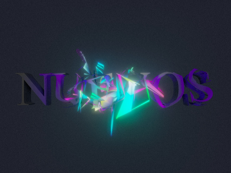
const text_geo = new TextGeometry("NUEVOS",{
    font:Resources.font,
    size:1.0,
    depth:0.2,
    bevelEnabled: true,
    bevelThickness: 0.1,
    bevelSize: 0.01,
    bevelOffset: 0,
    bevelSegments: 1
}); 

const mesh = new THREE.Mesh(
    text_geo,
    new THREE.MeshStandardMaterial({ 
        color: "#656565",
        metalness: 0.4, 
        roughness: 0.3
    })
);

scene.add(mesh);

By default, the origin of the text sits at (0, 0), but we want it centered.
To do that, we need to compute its BoundingBox and manually apply a translation to the geometry:

text_geo.computeBoundingBox();
const centerOffset = - 0.5 * ( text_geo.boundingBox.max.x - text_geo.boundingBox.min.x );
const centerOffsety = - 0.5 * ( text_geo.boundingBox.max.y - text_geo.boundingBox.min.y );
text_geo.translate( centerOffset, centerOffsety, 0 );

Now that we have the mesh and material ready, we can move on to the function that lets us blow everything up 💥

Three Shader Language

I really love TSL — it’s closed the gap between ideas and execution, in a context that’s not always the friendliest… shaders.

The effect we’re going to implement deforms the geometry’s vertices based on the pointer’s position, and uses spring physics to animate those deformations in a dynamic way.

But before we get to that, let’s grab a few attributes we’ll need to make everything work properly:

//  Original position of each vertex — we’ll use it as a reference
//  so unaffected vertices can "return" to their original spot
const initial_position = storage( text_geo.attributes.position, "vec3", count );

//  Normal of each vertex — we’ll use this to know which direction to "push" in
const normal_at = storage( text_geo.attributes.normal, "vec3", count );

//  Number of vertices in the geometry
const count = text_geo.attributes.position.count;

Next, we’ll create a storage buffer to hold the simulation data — and we’ll also write a function.
But not a regular JavaScript function — this one’s a compute function, written in the context of TSL.

It runs on the GPU and we’ll use it to set up the initial values for our buffers, getting everything ready for the simulation.

// In this buffer we’ll store the modified positions of each vertex —
// in other words, their current state in the simulation.
const   position_storage_at = storage(new THREE.StorageBufferAttribute(count,3),"vec3",count);   

const compute_init = Fn( ()=>{

	position_storage_at.element( instanceIndex ).assign( initial_position.element( instanceIndex ) );

} )().compute( count );

// Run the function on the GPU. This runs compute_init once per vertex.
renderer.computeAsync( compute_init );

Now we’re going to create another one of these functions — but unlike the previous one, this one will run inside the animation loop, since it’s responsible for updating the simulation on every frame.

This function runs on the GPU and needs to receive values from the outside — like the pointer position, for example.

To send that kind of data to the GPU, we use what’s called uniforms. They work like bridges between our “regular” code and the code that runs inside the GPU shader.

They’re defined like this:

const u_input_pos = uniform(new THREE.Vector3(0,0,0));
const u_input_pos_press = uniform(0.0);

With this, we can calculate the distance between the pointer position and each vertex of the geometry.

Then we clamp that value so the deformation only affects vertices within a certain radius.
To do that, we use the step function — it acts like a threshold, and lets us apply the effect only when the distance is below a defined value.

Finally, we use the vertex normal as a direction to push it outward.

const compute_update = Fn(() => {

    // Original position of the vertex — also its resting position
    const base_position = initial_position.element(instanceIndex);

    // The vertex normal tells us which direction to push
    const normal = normal_at.element(instanceIndex);

    // Current position of the vertex — we’ll update this every frame
    const current_position = position_storage_at.element(instanceIndex);

    // Calculate distance between the pointer and the base position of the vertex
    const distance = length(u_input_pos.sub(base_position));

    // Limit the effect's range: it only applies if distance is less than 0.5
    const pointer_influence = step(distance, 0.5).mul(1.0);

    // Compute the new displaced position along the normal.
    // Where pointer_influence is 0, there’ll be no deformation.
    const disorted_pos = base_position.add(normal.mul(pointer_influence));

    // Assign the new position to update the vertex
    current_position.assign(disorted_pos);

})().compute(count);

To make this work, we’re missing two key steps: we need to assign the buffer with the modified positions to the material, and we need to make sure the renderer runs the compute function on every frame inside the animation loop.

// Assign the buffer with the modified positions to the material
mesh.material.positionNode = position_storage_at.toAttribute();

// Animation loop
function animate() {
	// Run the compute function
	renderer.computeAsync(compute_update_0);

	// Render the scene
	renderer.renderAsync(scene, camera);
}

Right now the function doesn’t produce anything too exciting — the geometry moves around in a kinda clunky way. We’re about to bring in springs, and things will get much better.

// Spring — how much force we apply to reach the target value
velocity += (target_value - current_value) * spring;

// Friction controls the damping, so the movement doesn’t oscillate endlessly
velocity *= friction;

current_value += velocity;

But before that, we need to store one more value per vertex, the velocity, so let’s create another storage buffer.

const position_storage_at = storage(new THREE.StorageBufferAttribute(count, 3), "vec3", count);

// New buffer for velocity
const velocity_storage_at = storage(new THREE.StorageBufferAttribute(count, 3), "vec3", count);

const compute_init = Fn(() => {

    position_storage_at.element(instanceIndex).assign(initial_position.element(instanceIndex));
    
    // We initialize it too
    velocity_storage_at.element(instanceIndex).assign(vec3(0.0, 0.0, 0.0));

})().compute(count);

We’ll also add two uniforms: spring and friction.

const u_spring = uniform(0.05);
const u_friction = uniform(0.9);

Now we’ve implemented the springs in the update:

const compute_update = Fn(() => {

    const base_position = initial_position.element(instanceIndex);
    const current_position = position_storage_at.element(instanceIndex);

    // Get current velocity
    const current_velocity = velocity_storage_at.element(instanceIndex);

    const normal = normal_at.element(instanceIndex);

    const   distance =  length(u_input_pos.sub(base_position));
    const   pointer_influence = step(distance,0.5).mul(1.5);

    const disorted_pos = base_position.add(normal.mul(pointer_influence));
    disorted_pos.assign((mix(base_position, disorted_pos, u_input_pos_press)));
  
    // Spring implementation
    // velocity += (target_value - current_value) * spring;
    current_velocity.addAssign(disorted_pos.sub(current_position).mul(u_spring));
    // velocity *= friction;
    current_velocity.assign(current_velocity.mul(u_friction));
    // value += velocity
    current_position.addAssign(current_velocity);


})().compute(count);

Now we’ve got everything we need — time to start fine-tuning.

We’re going to add two things. First, we’ll use the TSL function mx_noise_vec3 to generate some noise for each vertex. That way, we can tweak the direction a bit so things don’t feel so stiff.

We’re also going to rotate the vertices using another TSL function — surprise, it’s called rotate.

Here’s what our updated compute_update function looks like:

const compute_update = Fn(() => {

    const base_position = initial_position.element(instanceIndex);
    const current_position = position_storage_at.element(instanceIndex);
    const current_velocity = velocity_storage_at.element(instanceIndex);

    const normal = normal_at.element(instanceIndex);

    // NEW: Add noise so the direction in which the vertices "explode" isn’t too perfectly aligned with the normal
    const noise = mx_noise_vec3(current_position.mul(0.5).add(vec3(0.0, time, 0.0)), 1.0).mul(u_noise_amp);

    const distance = length(u_input_pos.sub(base_position));
    const pointer_influence = step(distance, 0.5).mul(1.5);

    const disorted_pos = base_position.add(noise.mul(normal.mul(pointer_influence)));

    // NEW: Rotate the vertices to give the animation a more chaotic feel
    disorted_pos.assign(rotate(disorted_pos, vec3(normal.mul(distance)).mul(pointer_influence)));

    disorted_pos.assign(mix(base_position, disorted_pos, u_input_pos_press));

    current_velocity.addAssign(disorted_pos.sub(current_position).mul(u_spring));
    current_position.addAssign(current_velocity);
    current_velocity.assign(current_velocity.mul(u_friction));

})().compute(count);

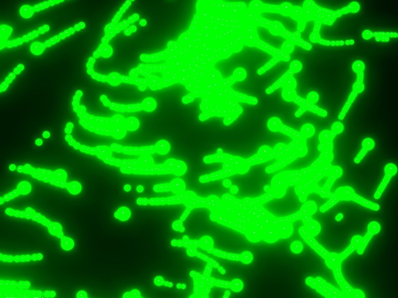
Now that the motion feels right, it’s time to tweak the material colors a bit and add some post-processing to the scene.

We’re going to work on the emissive color — meaning it won’t be affected by lights, and it’ll always look bright and explosive. Especially once we throw some bloom on top. (Yes, bloom everything.)

We’ll start from a base color (whichever you like), passed in as a uniform. To make sure each vertex gets a slightly different color, we’ll offset its hue a bit using values from the buffers — in this case, the velocity buffer.

The hue function takes a color and a value to shift its hue, kind of like how offsetHSL works in THREE.Color.

// Base emissive color
const emissive_color = color(new THREE.Color("0000ff"));

const vel_at = velocity_storage_at.toAttribute();
const hue_rotated = vel_at.mul(Math.PI*10.0);

// Multiply by the length of the velocity buffer — this means the more movement,
// the more the vertex color will shift
const emission_factor = length(vel_at).mul(10.0);

// Assign the color to the emissive node and boost it as much as you want
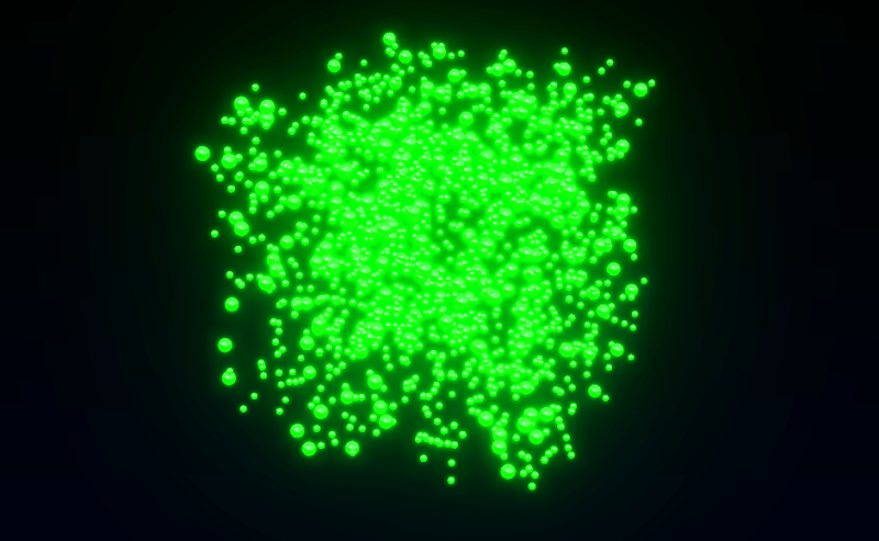
mesh.material.emissiveNode = hue(emissive_color, hue_rotated).mul(emission_factor).mul(5.0);

Finally! Lets change scene background color and add Fog:

scene.fog = new THREE.Fog(new THREE.Color("#41444c"),0.0,8.5);
scene.background = scene.fog.color;

Now, let’s spice up the scene with a bit of post-processing — one of those things that got way easier to implement thanks to TSL.

We’re going to include three effects: ambient occlusion, bloom, and noise. I always like adding some noise to what I do — it helps break up the flatness of the pixels a bit.

I won’t go too deep into this part — I grabbed the AO setup from the Three.js examples.

const   composer = new THREE.PostProcessing(renderer);
const   scene_pass = pass(scene,camera);

scene_pass.setMRT(mrt({
    output:output,
    normal:normalView
}));

const   scene_color = scene_pass.getTextureNode("output");
const   scene_depth = scene_pass.getTextureNode("depth");
const   scene_normal = scene_pass.getTextureNode("normal");

const ao_pass = ao( scene_depth, scene_normal, camera);
ao_pass.resolutionScale = 1.0;

const   ao_denoise = denoise(ao_pass.getTextureNode(), scene_depth, scene_normal, camera ).mul(scene_color);
const   bloom_pass = bloom(ao_denoise,0.3,0.2,0.1);
const   post_noise = (mx_noise_float(vec3(uv(),time.mul(0.1)).mul(sizes.width),0.03)).mul(1.0);

composer.outputNode = ao_denoise.add(bloom_pass).add(post_noise);

Alright, that’s it amigas — thanks so much for reading, and I hope it was useful!