برچسب: useful

  • XGBoost for beginners – from CSV to Trustworthy Model – Useful code


    import numpy as np

    import pandas as pd

    import xgboost as xgb


    from sklearn.model_selection import train_test_split

    from sklearn.metrics import (

        confusion_matrix, precision_score, recall_score,

        roc_auc_score, average_precision_score, precision_recall_curve

    )


    # 1) Load a tiny cusomer churn CSV called churn.csv 

    df = pd.read_csv(“churn.csv”)


    # 2) Do quick, safe checks – missing values and class balance.

    missing_share = df.isna().mean().sort_values(ascending=False)

    class_share = df[“churn”].value_counts(normalize=True).rename(“share”)

    print(“Missing share (top 5):\n”, missing_share.head(5), “\n”)

    print(“Class share:\n”, class_share, “\n”)


    # 3) Split data into train, validation, test – 60-20-20.

    X = df.drop(columns=[“churn”]); y = df[“churn”]

    X_tr, X_te, y_tr, y_te = train_test_split(X, y, test_size=0.20, stratify=y, random_state=13)

    X_tr, X_va, y_tr, y_va = train_test_split(X_tr, y_tr, test_size=0.25, stratify=y_tr, random_state=13)

    neg, pos = int((y_tr==0).sum()), int((y_tr==1).sum())

    spw = neg / max(pos, 1)

    print(f“Shapes -> train {X_tr.shape}, val {X_va.shape}, test {X_te.shape}”)

    print(f“Class balance in train -> neg {neg}, pos {pos}, scale_pos_weight {spw:.2f}\n”)


    # Wrap as DMatrix (fast internal format)

    feat_names = list(X.columns)

    dtr = xgb.DMatrix(X_tr, label=y_tr, feature_names=feat_names)

    dva = xgb.DMatrix(X_va, label=y_va, feature_names=feat_names)

    dte = xgb.DMatrix(X_te, label=y_te, feature_names=feat_names)


    # 4) Train XGBoost with early stopping using the Booster API.

    params = dict(

        objective=“binary:logistic”,

        eval_metric=“aucpr”,

        tree_method=“hist”,

        max_depth=5,

        eta=0.03,

        subsample=0.8,

        colsample_bytree=0.8,

        reg_lambda=1.0,

        scale_pos_weight=spw

    )

    bst = xgb.train(params, dtr, num_boost_round=4000, evals=[(dva, “val”)],

                    early_stopping_rounds=200, verbose_eval=False)

    print(“Best trees (baseline):”, bst.best_iteration)


    # 6) Choose a practical decision treshold from validation – “a line in the sand”.

    p_va = bst.predict(dva, iteration_range=(0, bst.best_iteration + 1))

    pre, rec, thr = precision_recall_curve(y_va, p_va)

    f1 = 2 * pre * rec / np.clip(pre + rec, 1e9, None)

    t_best = float(thr[np.argmax(f1[:1])])

    print(“Chosen threshold t_best (validation F1):”, round(t_best, 3), “\n”)


    # 7) Explain results on the test set in plain terms – confusion matrix, precision, recall, ROC AUC, PR AUC

    p_te = bst.predict(dte, iteration_range=(0, bst.best_iteration + 1))

    pred = (p_te >= t_best).astype(int)

    cm = confusion_matrix(y_te, pred)

    print(“Confusion matrix:\n”, cm)

    print(“Precision:”, round(precision_score(y_te, pred), 3))

    print(“Recall   :”, round(recall_score(y_te, pred), 3))

    print(“ROC AUC  :”, round(roc_auc_score(y_te, p_te), 3))

    print(“PR  AUC  :”, round(average_precision_score(y_te, p_te), 3), “\n”)


    # 8) See which column mattered most

    # (a hint – if people start calling the call centre a lot, most probably there is a problem and they will quit using your service)

    imp = pd.Series(bst.get_score(importance_type=“gain”)).sort_values(ascending=False)

    print(“Top features by importance (gain):\n”, imp.head(10), “\n”)


    # 9) Add two business rules with monotonic constraints

    cons = [0]*len(feat_names)

    if “debt_ratio” in feat_names: cons[feat_names.index(“debt_ratio”)] = 1     # non-decreasing

    if “tenure_months” in feat_names: cons[feat_names.index(“tenure_months”)] = 1  # non-increasing

    mono = “(“ + “,”.join(map(str, cons)) + “)”


    params_cons = params.copy()

    params_cons.update({“monotone_constraints”: mono, “max_bin”: 512})


    bst_cons = xgb.train(params_cons, dtr, num_boost_round=4000, evals=[(dva, “val”)],

                         early_stopping_rounds=200, verbose_eval=False)

    print(“Best trees (constrained):”, bst_cons.best_iteration)


    # 10) Compare the quality of bst_cons and bst with a few lines.

    p_cons = bst_cons.predict(dte, iteration_range=(0, bst_cons.best_iteration + 1))

    print(“PR AUC  baseline vs constrained:”, round(average_precision_score(y_te, p_te), 3),

          “vs”, round(average_precision_score(y_te, p_cons), 3))

    print(“ROC AUC baseline vs constrained:”, round(roc_auc_score(y_te, p_te), 3),

          “vs”, round(roc_auc_score(y_te, p_cons), 3), “\n”)


    # 11) Save both models

    bst.save_model(“easy_xgb_base.ubj”)

    bst_cons.save_model(“easy_xgb_cons.ubj”)

    print(“Saved models: easy_xgb_base.ubj, easy_xgb_cons.ubj”)


    Source link

  • Correlation – explained with Python – Useful code


    When you plot two variables, you see data dots scattered across the plane. Their overall tilt and shape tell you how the variables move together. Correlation turns that visual impression into a single number you can report and compare.

    What correlation measures

    Correlation summarises the direction and strength of association between two numeric variables on a scale from −1 to +1.

    • Sign shows direction
      • positive – larger x tends to come with larger y
      • negative – larger x tends to come with smaller y
    • Magnitude shows strength
      • near 0 – weak association
      • near 1 in size – strong association

    Correlation does not prove causation.

    Two methods to measure correlation

    Pearson correlation – distance based

    Pearson asks: how straight is the tilt of the data dots? It uses actual distances from a straight line, so it is excellent for line-like patterns and sensitive to outliers. Use when:

    • you expect a roughly straight relationship
    • units and distances matter
    • residuals look symmetric around a line

    Spearman correlation – rank based

    Spearman converts each variable to ranks (1st, 2nd, 3rd, …) and then computes Pearson on those ranks. It measures monotonic association: do higher x values tend to come with higher y values overall, even if the shape is curved.

    Ranks ignore distances and care only about order, which gives two benefits:

    • robust to outliers and weird units
    • invariant to any monotonic transform (log, sqrt, min-max), since order does not change

    Use when:

    • you expect a consistent up or down trend that may be curved
    • the data are ordinal or have many ties
    • outliers are a concern

    r and p in plain language

    • r is the correlation coefficient. It is your effect size on the −1 to +1 scale.
    • p answers: if there were truly no association, how often would we see an r at least this large in magnitude just by random chance.

    Small p flags statistical signal. It is not a measure of importance. Usually findings, where p is bigger than .05 should be ignored.

    When Pearson and Spearman disagree?

    • Curved but monotonic (for example price vs horsepower with diminishing returns)
      Spearman stays high because order increases consistently. Pearson is smaller because a straight line underfits the curve.

    • Outliers (for example a 10-year-old exotic priced very high)
      Pearson can jump because distances change a lot. Spearman changes less because rank order barely changes.

    https://www.youtube.com/watch?v=IdffxjPdNJY

    Jupyter Notebook in GitHub with code from the video above.

    Enjoy it! 🙂


    Source link

  • Python – Learn Pandas with SQL Examples – Football Analytics Example – Useful code

    Python – Learn Pandas with SQL Examples – Football Analytics Example – Useful code


    When working with data, you will often move between SQL databases and Pandas DataFrames. SQL is excellent for storing and retrieving data, while Pandas is ideal for analysis inside Python.

    In this article, we show how both can be used together, using a football (soccer) mini-league dataset. We build a small SQLite database in memory, read the data into Pandas, and then solve real analytics questions.

    There are neither pythons or pandas in Bulgaria. Just software.

    • Setup – SQLite and Pandas

    We start by importing the libraries and creating three tables –
    [teams, players, matches]  inside an SQLite in-memory database.

    Now, we have three tables.

    • Loading SQL Data into Pandas


    pd.read_sql  does the magic to load either a table or a custom query directly.

    At this point, the SQL data is ready for analysis with Pandas.

    • SQL vs Pandas – Filtering Rows

    Task: Find forwards (FW) with more than 1200 minutes on the field:

    SQL:

    Pandas:

    As expected, both return the same subset, one written in SQL and the other in Pandas.

    Task: Total goals per team:

    SQL:

    Pandas:

    Both results show which team has scored more goals overall.

    Task: Add the city of each team to the players table.

    SQL:

    Pandas:

    The fun part: calculating points (3 for a win, 1 for a draw) and goal difference. Only with SQL this time.

    This produces a proper football league ranking – teams sorted by points and then goal difference:

    • Quick Pandas Tricks

      • Top scorers with
        nlargest:

    https://www.youtube.com/watch?v=U0lbBaHFAEM

    https://github.com/Vitosh/Python_personal/tree/master/YouTube/041_Python-Learn-Pandas-with-Football-Analytics


    Source link

  • Docker + Python CRUD API + Excel VBA – All for beginners – Useful code


    import os, sqlite3

    from typing import List, Optional

    from fastapi import FastAPI, HTTPException

    from pydantic import BaseModel


    DB_PATH = os.getenv(“DB_PATH”, “/data/app.db”)  


    app = FastAPI(title=“Minimal Todo CRUD”, description=“Beginner-friendly, zero frontend.”)


    class TodoIn(BaseModel):

        title: str

        completed: bool = False


    class TodoUpdate(BaseModel):

        title: Optional[str] = None

        completed: Optional[bool] = None


    class TodoOut(TodoIn):

        id: int


    def row_to_todo(row) -> TodoOut:

        return TodoOut(id=row[“id”], title=row[“title”], completed=bool(row[“completed”]))


    def get_conn():

        conn = sqlite3.connect(DB_PATH)

        conn.row_factory = sqlite3.Row

        return conn


    @app.on_event(“startup”)

    def init_db():

        os.makedirs(os.path.dirname(DB_PATH), exist_ok=True)

        conn = get_conn()

        conn.execute(“””

            CREATE TABLE IF NOT EXISTS todos(

                id INTEGER PRIMARY KEY AUTOINCREMENT,

                title TEXT NOT NULL,

                completed INTEGER NOT NULL DEFAULT 0

            )

        “””)

        conn.commit(); conn.close()


    @app.post(“/todos”, response_model=TodoOut, status_code=201)

    def create_todo(payload: TodoIn):

        conn = get_conn()

        cur = conn.execute(

            “INSERT INTO todos(title, completed) VALUES(?, ?)”,

            (payload.title, int(payload.completed))

        )

        conn.commit()

        row = conn.execute(“SELECT * FROM todos WHERE id=?”, (cur.lastrowid,)).fetchone()

        conn.close()

        return row_to_todo(row)


    @app.get(“/todos”, response_model=List[TodoOut])

    def list_todos():

        conn = get_conn()

        rows = conn.execute(“SELECT * FROM todos ORDER BY id DESC”).fetchall()

        conn.close()

        return [row_to_todo(r) for r in rows]


    @app.get(“/todos/{todo_id}”, response_model=TodoOut)

    def get_todo(todo_id: int):

        conn = get_conn()

        row = conn.execute(“SELECT * FROM todos WHERE id=?”, (todo_id,)).fetchone()

        conn.close()

        if not row:

            raise HTTPException(404, “Todo not found”)

        return row_to_todo(row)


    @app.patch(“/todos/{todo_id}”, response_model=TodoOut)

    def update_todo(todo_id: int, payload: TodoUpdate):

        data = payload.model_dump(exclude_unset=True)

        if not data:

            return get_todo(todo_id)  # nothing to change


        fields, values = [], []

        if “title” in data:

            fields.append(“title=?”); values.append(data[“title”])

        if “completed” in data:

            fields.append(“completed=?”); values.append(int(data[“completed”]))

        if not fields:

            return get_todo(todo_id)


        conn = get_conn()

        cur = conn.execute(f“UPDATE todos SET {‘, ‘.join(fields)} WHERE id=?”, (*values, todo_id))

        if cur.rowcount == 0:

            conn.close(); raise HTTPException(404, “Todo not found”)

        conn.commit()

        row = conn.execute(“SELECT * FROM todos WHERE id=?”, (todo_id,)).fetchone()

        conn.close()

        return row_to_todo(row)


    @app.delete(“/todos/{todo_id}”, status_code=204)

    def delete_todo(todo_id: int):

        conn = get_conn()

        cur = conn.execute(“DELETE FROM todos WHERE id=?”, (todo_id,))

        conn.commit(); conn.close()

        if cur.rowcount == 0:

            raise HTTPException(404, “Todo not found”)

        return  # 204 No Content


    Source link

  • Exploring SOAP Web Services – From Browser Console to Python – Useful code

    Exploring SOAP Web Services – From Browser Console to Python – Useful code


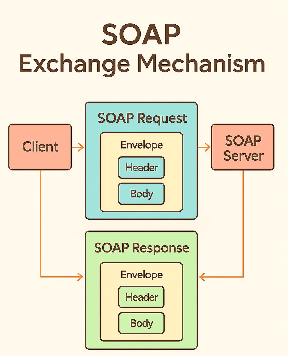
    SOAP (Simple Object Access Protocol) might sound intimidating (or funny) but it is actually a straightforward way for systems to exchange structured messages using XML. In this article, I am introducing SOAP through YouTube video, where it is explored through 2 different angles – first in the Chrome browser console, then with Python and Jupyter Notebook.

    The SOAP Exchange Mechanism uses requests and response.

    Part 1 – Soap in the Chrome Browser Console

    We start by sending SOAP requests directly from the browser’s JS console. This is a quick way to see the raw XML
    <soap>  envelopes in action. Using a public integer calculator web service, we perform basic operations – additions, subtraction, multiplication, division – and observe how the requests and responses happen in real time!

    For the browser, the entire SOAP journey looks like that:

    Chrome Browser -> HTTP POST -> SOAP XML -> Server (http://www.dneonline.com/calculator.asmx?WSDL) -> SOAP XML -> Chrome Browser

    A simple way to call it is with constants, to avoid the strings:

    Like that:

    Part 2 – Soap with Python and Jupyter Notebook

    Here we jump into Python. With the help of libaries, we load the the WSDL (Web Services Description Language) file, inspect the available operations, and call the same calculator service programmatically.


    https://www.youtube.com/watch?v=rr0r1GmiyZg
    Github code – https://github.com/Vitosh/Python_personal/tree/master/YouTube/038_Python-SOAP-Basics!

    Enjoy it! 🙂


    Source link

  • Shortest route between points in a city – with Python and OpenStreetMap – Useful code

    Shortest route between points in a city – with Python and OpenStreetMap – Useful code


    After the article for introduction to Graphs in Python, I have decided to put the graph theory into practice and start looking for the shortest points between points in a city. Parts of the code are inspired from the book Optimization Algorithms by Alaa Khamis, other parts are mine 🙂

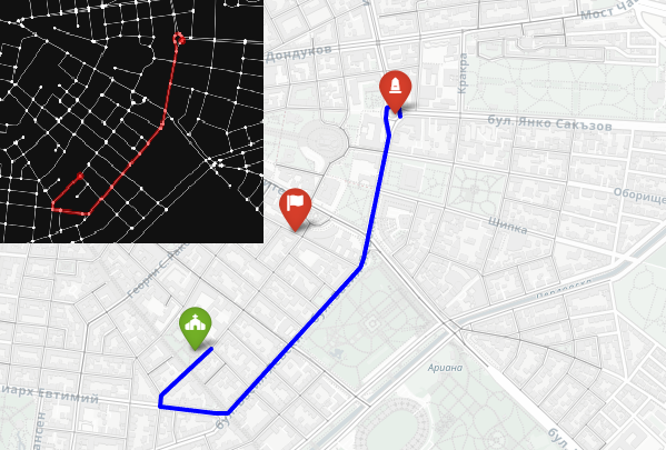
    The idea is to go from the monument to the church with a car. The flag marks the middle, between the two points.

    The solution uses several powerful Python libraries:

    • OSMnx to download and work with real road networks from OpenStreetMap
    • NetworkX to model the road system as a graph and calculate the shortest path using Dijkstra’s algorithm
    • Folium for interactive map visualization

    We start by geocoding the two landmarks to get their latitude and longitude. Then we build a drivable street network centered around the Levski Monument using ox.graph_from_address. After snapping both points to the nearest graph nodes, we compute the shortest route by distance. Finally, we visualize everything both in an interactive map and in a clean black-on-white static graph where the path is drawn in yellow.


    Nodes and edges in radius of 1000 meters around the center point


    Red and green are the nodes, that are the closest to the start and end points.


    The closest driving route between the two points is in blue.

    The full code is implemented in a Jupyter Notebook in GitHub and explained in the video.

    https://www.youtube.com/watch?v=kQIK2P7erAA

    GitHub link:

    Enjoy the rest of your day! 🙂


    Source link

  • Introduction to Graphs in Python – Useful code

    Introduction to Graphs in Python – Useful code


    Lately, I am reading the book Optimization Algorithms by Alaa Khamis and the chapter 3 – Blind Search Algorithms, has caught my attention. The chapter starts with explaining what graphs are how these are displayed in python and I have decided to make a YT video, presenting the code of the book with Jupyter Notebook.

    Trees are different, when we talk about graphs in python

    Why graphs? Because they are everywhere:

    • A road map is a graph
    • Your social-media friends form a graph
    • Tasks in a to-do list, with dependables on each other, can be a graph

    With Python we can build and draw these structures in just a few lines of code.

    Setup

    Undirected graph

    • Edges have no arrows
    • Use it for two‑way streets or mutual friendships.

    Undirected graph

    Directed graph

    • Arrowheads show direction.
    • Good for “A follows B” but not the other way around.

    Directed graph

    Multigraph

    • Allows two or more edges between the same nodes.
    • Think of two train lines that join the same pair of cities.

    Multigraph

    Directed Acyclic Graph (Tree)

    • No cycles = no way to loop back.
    • Used in task schedulers and Git histories.

    Directed Acyclic Graph (Tree)

    Hypergraph

    • One “edge” can touch many nodes.
    • We simulate it with a bipartite graph: red squares = hyper‑edges.

    Hypergraph

    Weighted Graph

    • Graph with weights on the edges
    • Idea for mapping distances between cities on a map

    Weighted Graph

    https://www.youtube.com/watch?v=8vnu_5QRC74

    🙂


    Source link

  • Python – Solving 7 Queen Problem with Tabu Search – Useful code

    Python – Solving 7 Queen Problem with Tabu Search – Useful code


    The n-queens problem is a classic puzzle that involves placing n chess queens on an n × n chessboard in such a way that no two queens threaten each other. In other words,
    no two queens should share the same row, column, or diagonal. This is a constraintsatisfaction problem (CSP) that does not define an explicit objective function. Let’s
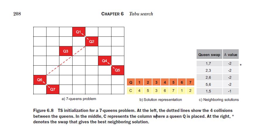
    suppose we are attempting to solve a 7-queens problem using tabu search. In this problem, the number of collisions in the initial random configuration shown in figure 6.8a is 4: {Q1– Q2}, {Q2– Q6}, {Q4– Q5}, and {Q6– Q7}.

    The above is part of the book Optimization Algorithms by Alaa Khamis, which I have used as a stepstone, in order to make a YT video, explaining the core of the tabu search with the algorithm. The solution of the n-queens problem is actually interesting, as its idea is to swap queen’s columns until these are allowed to be swaped and until the constrains are solved. The “tabu tenure” is just a type of record, that does not allow a certain change to be carried for a number of moves after it has been carried out. E.g., once you replace the columns of 2 queens, you are not allowed to do the same for the next 3 moves. This allows you to avoid loops.

    https://www.youtube.com/watch?v=m7uAw3cNMAM

    Github code:

    Thank you and have a nice day! 🙂


    Source link

  • VBA – A* Search Algorithm with Excel – Useful code


    Ok, so some 10 years ago, I was having fun coding A* Search Algorithms in Excel in VitoshAcademy and this is what I had built back then:

    VBA – A* search algorithm with Excel – Really?

    VBA – A Search Algorithm with VBA – Teil Zwei

    The second one is actually quite fun and I had forgotten about it. Today, I will present a third one, that has a few more features, namely the following:

    • It can be copied completely into a blank Excel’s VBA module, without any additional setup and it will work
    • You can choose for distance method (Manhattan or Heuristics)
    • You can choose for displaying or not calculations in Excel (
      writeScores = False )
    • You can
      ResetAndKeep() , which cleans out the maze, but keeps the obstacles
    • You can setup your own start and goal cell. By simply writing
      s and
      g , somewhere in the PLAYGROUND.
    • You can change the speed of writing in the Excel file, by changing the
      delay variable.

    These are the current commands:


    Source link

  • Rule of 72 – Useful code

    Rule of 72 – Useful code


    Ever heard of the Rule of 72? It’s a classic finance shortcut that tells you how many years it takes for an investment to double at a given interest rate—without reaching for a calculator! Pretty much, if you want to understand when you are going to double your money, that are growing with 7% per year, then simply divide 72 by 7 and see the approximate answer. It works like that and it is approximately ok, for values between 5 and 10%.

    For all other values, the formula looks like this:

    ln(2) is approximately 0.693. Hence, it is 0.693 divided by ln(1+tiny percentage).

    With Python the formula looks like this:

    If you want to see how exact the formula is, then a good comparison vs the exact value looks like this:

    The execution of the code from above like this:

    The YT video, explaining the code and is here:

    https://www.youtube.com/watch?v=BURstTrQWkA

    The GitHub code is here: https://github.com/Vitosh/Python_personal/tree/master/YouTube/023_Python-Rule-of-72

    A nice picture from Polovrak Peak, Bulgaria

    Enjoy!


    Source link