Just a second! 🫷 If you are here, it means that you are a software developer.
So, you know that storage, networking, and domain management have a cost .
If you want to support this blog, please ensure that you have disabled the adblocker for this site. I configured Google AdSense to show as few ADS as possible – I don’t want to bother you with lots of ads, but I still need to add some to pay for the resources for my site.
Thank you for your understanding. – Davide
From C# 6 on, you can use the when keyword to specify a condition before handling an exception.
Consider this – pretty useless, I have to admit – type of exception:
publicclassRandomException : System.Exception
{
publicint Value { get; }
public RandomException()
{
Value = (new Random()).Next();
}
}
This exception type contains a Value property which is populated with a random value when the exception is thrown.
What if you want to print a different message depending on whether the Value property is odd or even?
You can do it this way:
try{
thrownew RandomException();
}
catch (RandomException re)
{
if(re.Value % 2 == 0)
Console.WriteLine("Exception with even value");
else Console.WriteLine("Exception with odd value");
}
But, well, you should keep your catch blocks as simple as possible.
That’s where the when keyword comes in handy.
CSharp when clause
You can use it to create two distinct catch blocks, each one of them handles their case in the cleanest way possible.
try{
thrownew RandomException();
}
catch (RandomException re) when (re.Value % 2 == 0)
{
Console.WriteLine("Exception with even value");
}
catch (RandomException re)
{
Console.WriteLine("Exception with odd value");
}
You must use the when keyword in conjunction with a condition, which can also reference the current instance of the exception being caught. In fact, the condition references the Value property of the RandomException instance.
A real usage: HTTP response errors
Ok, that example with the random exception is a bit… useless?
Let’s see a real example: handling different HTTP status codes in case of failing HTTP calls.
In the following snippet, I call an endpoint that returns a specified status code (506, in my case).
try{
var endpoint = "https://mock.codes/506";
var httpClient = new HttpClient();
var response = await httpClient.GetAsync(endpoint);
response.EnsureSuccessStatusCode();
}
catch (HttpRequestException ex) when (ex.StatusCode == (HttpStatusCode)506)
{
Console.WriteLine("Handle 506: Variant also negotiates");
}
catch (HttpRequestException ex)
{
Console.WriteLine("Handle another status code");
}
If the response is not a success, the response.EnsureSuccessStatusCode() throws an exception of type HttpRequestException. The thrown exception contains some info about the returned status code, which we can use to route the exception handling to the correct catch block using when (ex.StatusCode == (HttpStatusCode)506).
When working with data, you will often move between SQL databases and Pandas DataFrames. SQL is excellent for storing and retrieving data, while Pandas is ideal for analysis inside Python.
In this article, we show how both can be used together, using a football (soccer) mini-league dataset. We build a small SQLite database in memory, read the data into Pandas, and then solve real analytics questions.
There are neither pythons or pandas in Bulgaria. Just software.
Setup – SQLite and Pandas
We start by importing the libraries and creating three tables –
[teams,players,matches] inside an SQLite in-memory database.
1
2
3
4
5
6
7
8
9
10
11
12
13
14
15
16
17
18
19
20
21
22
23
24
25
26
27
28
29
30
31
32
33
34
35
36
37
38
39
40
41
42
43
44
45
46
47
48
49
50
51
52
53
54
55
56
57
importsqlite3
importpandas aspd
importnumpy asnp
conn=sqlite3.connect(“:memory:”)
cur=conn.cursor()
cur.executescript(“””
DROP TABLE IF EXISTS teams;
DROP TABLE IF EXISTS players;
DROP TABLE IF EXISTS matches;
CREATE TABLE teams (
team TEXT PRIMARY KEY,
city TEXT NOT NULL,
founded INTEGER NOT NULL
);
CREATE TABLE players (
player_id INTEGER PRIMARY KEY AUTOINCREMENT,
name TEXT NOT NULL,
team TEXT NOT NULL REFERENCES teams(team),
pos TEXT NOT NULL,
age INTEGER NOT NULL,
goals INTEGER NOT NULL,
assists INTEGER,
minutes INTEGER NOT NULL
);
CREATE TABLE matches (
match_id INTEGER PRIMARY KEY AUTOINCREMENT,
date TEXT NOT NULL,
home TEXT NOT NULL,
away TEXT NOT NULL,
home_goals INTEGER NOT NULL,
away_goals INTEGER NOT NULL
);
INSERT INTO teams(team, city, founded) VALUES
(‘Lions’,’Sofia’, 2015),
(‘Wolves’,’Plovdiv’,1914),
(‘Eagles’,’Varna’,1930);
INSERT INTO players(name, team, pos, age, goals, assists, minutes) VALUES
(‘Ivan Petrov’,’Lions’,’FW’,24,11,3,1350),
(‘Martin Kolev’,’Lions’,’MF’,29,4,NULL,1490),
(‘Rui Costa’,’Lions’,’DF’,31,1,2,1600),
(‘Georgi Iliev’,’Wolves’,’FW’,27,7,5,1410),
(‘Joe Jackson’,’Wolves’,’FW’,27,17,5,410),
(‘Peter Marin’,’Eagles’,’FW’,20,5,1,870);
INSERT INTO matches(date,home,away,home_goals,away_goals) VALUES
(‘2024-08-03′,’Lions’,’Wolves’,2,1),
(‘2024-08-10′,’Eagles’,’Lions’,1,3),
(‘2024-08-17′,’Wolves’,’Eagles’,2,2);
“””)
conn.commit()
Now, we have three tables.
Loading SQL Data into Pandas
pd.read_sql does the magic to load either a table or a custom query directly.
teams=pd.read_sql(“SELECT * FROM teams”,conn)
players=pd.read_sql(“SELECT * FROM players”,conn)
matches=pd.read_sql(“SELECT * FROM matches”,conn,parse_dates=[“date”])
print(teams)
print(players.head())
print(matches)
At this point, the SQL data is ready for analysis with Pandas.
SQL vs Pandas – Filtering Rows
Task: Find forwards (FW) with more than 1200 minutes on the field:
Just a second! 🫷 If you are here, it means that you are a software developer.
So, you know that storage, networking, and domain management have a cost .
If you want to support this blog, please ensure that you have disabled the adblocker for this site. I configured Google AdSense to show as few ADS as possible – I don’t want to bother you with lots of ads, but I still need to add some to pay for the resources for my site.
Thank you for your understanding. – Davide
Things that depend on concrete stuff are difficult to use when testing. Think of the file system: to have tests work properly, you have to ensure that the file system is structured exactly as you are expecting it to be.
A similar issue occurs with dates: if you create tests based on the current date, they will fail the next time you run them.
In short, you should find a way to abstract these functionalities, to make them usable in the tests.
In this article, we are going to focus on the handling of dates: we’ll learn what the TimeProvider class is, how to use it and how to mock it.
The old way for handling dates: a custom interface
Back in the days, the most straightforward approach to add abstraction around the date management was to manually create an interface, or an abstract class, to wrap the access to the current date:
Easy: you then have to add an instance of it in the DI engine, and you are good to go.
The only problem? You have to do it for every project you are working on. Quite a waste of time!
How to use TimeProvider in a .NET application to get the current date
Along with .NET 8, the .NET team released an abstract class named TimeProvider. This abstract class, beyond providing an abstraction for local time, exposes methods for working with high-precision timestamps and TimeZones.
It’s important to notice that dates are returned as DateTimeOffset, and not as DateTime instances.
TimeProvider comes out-of-the-box with a .NET Console application, accessible as a singleton:
staticvoid Main(string[] args)
{
Console.WriteLine("Hello, World!");
DateTimeOffset utc = TimeProvider.System.GetUtcNow();
Console.WriteLine(utc);
DateTimeOffset local = TimeProvider.System.GetLocalNow();
Console.WriteLine(local);
}
On the contrary, if you need to use Dependency Injection, for example, in .NET APIs, you have to inject it as a singleton, like this:
Now, how can we test the ItsVacationTime of the SummerVacationCalendar class?
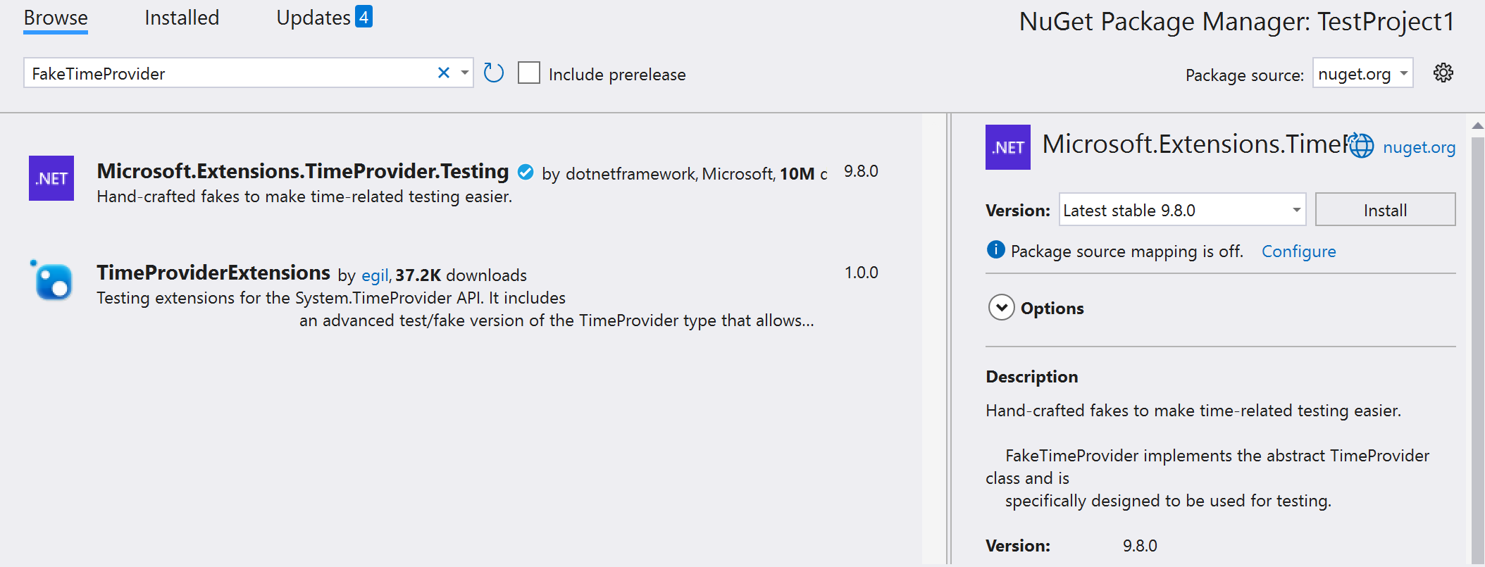
We can use the Microsoft.Extensions.TimeProvider.Testing NuGet library, still provided by Microsoft, which provides a FakeTimeProvider class that acts as a stub for the TimeProvider abstract class:
By using the FakeTimeProvider class, you can set the current UTC and Local time, as well as configure the other options provided by TimeProvider.
Here’s an example:
[Fact]publicvoid WhenItsAugust_ShouldReturnTrue()
{
// Arrangevar fakeTime = new FakeTimeProvider();
fakeTime.SetUtcNow(new DateTimeOffset(2025, 8, 14, 22, 24, 12, TimeSpan.Zero));
var sut = new SummerVacationCalendar(fakeTime);
// Actvar isVacation = sut.ItsVacationTime();
// Assert Assert.True(isVacation);
}
[Fact]publicvoid WhenItsNotAugust_ShouldReturnFalse()
{
// Arrangevar fakeTime = new FakeTimeProvider();
fakeTime.SetUtcNow(new DateTimeOffset(2025, 3, 14, 22, 24, 12, TimeSpan.Zero));
var sut = new SummerVacationCalendar(fakeTime);
// Actvar isVacation = sut.ItsVacationTime();
// Assert Assert.False(isVacation);
}
Further readings
Actually, TimeProvider provides way more functionalities than just returning the UTC and the Local time.
Maybe we’ll explore them in the future. But for now, do you know how the DateTimeKind enumeration impacts the way you create new DateTimes?
However, always remember to test the code not against the actual time but against static values. But, if for some reason you cannot add TimeProvider in your classes, there are other less-intrusive strategies that you can use (and that can work for other types of dependencies as well, like the file system):
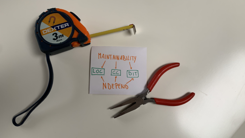
Keeping an eye on maintainability is mandatory for every project which should live long. With NDepend, you can measure maintainability for .NET projects.
Table of Contents
Just a second! 🫷 If you are here, it means that you are a software developer.
So, you know that storage, networking, and domain management have a cost .
If you want to support this blog, please ensure that you have disabled the adblocker for this site. I configured Google AdSense to show as few ADS as possible – I don’t want to bother you with lots of ads, but I still need to add some to pay for the resources for my site.
Thank you for your understanding. – Davide
Software systems can be easy to build, but hard to maintain. The more a system will be maintained, the more updates to the code will be needed.
Structuring the code to help maintainability is crucial if your project is expected to evolve.
In this article, we will learn how to measure the maintainability of a .NET project using NDepend, a tool that can be installed as an extension in Visual Studio.
So, let’s begin with the how, and then we’ll move to the what.
Introducing NDepend
NDepend is a tool that performs static analysis on any .NET project.
It is incredibly powerful and can calculate several metrics that you can use to improve the quality of your code, like Lines of Code, Cyclomatic Complexity, and Coupling.
You can use NDepend in two ways: installing it on your local Visual Studio instance, or using it in your CI/CD pipelines, to generate reports during the build process.
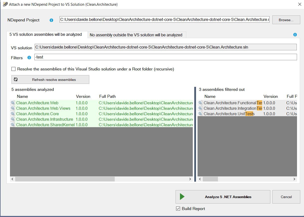
In this article, I’ve installed it as a Visual Studio extension. Once it is ready, you’ll have to create a new NDepend project and link it to your current solution.
To do that, click on the ⚪ icon on the bottom-right corner of Visual Studio, and create a new NDepend project. It will create a ndproj project and attach it to your solution.
When creating a new NDepend project, you can choose which of your .NET projects must be taken into consideration. You’ll usually skip analyzing test projects.
Then, to run the analysis of your solution, you need to click again on that ⚪ icon and click Run analysis and generate report.
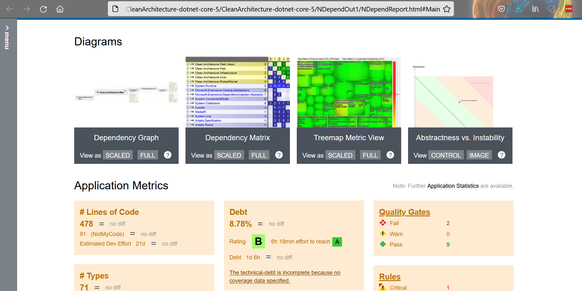
Now you’ll have two ways to access the results. On an HTML report, like this one:
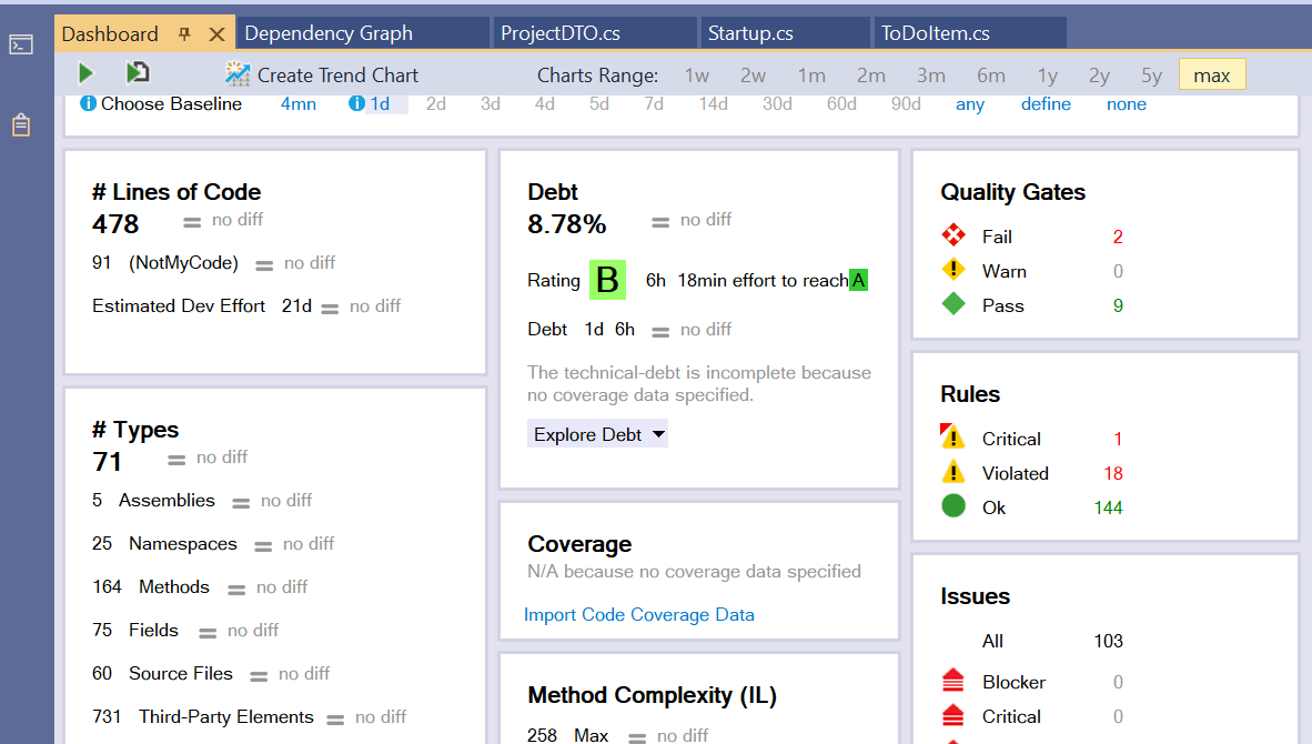
Or as a Dashboard integrated with Visual Studio:
You will find most of the things in the HTML report.
What is Maintainability
Maintainability is a quality of a software system (a single application or a group of applications) that describes how easy it is to maintain it.
Easy-to-maintain code has many advantages:
it allows quicker and less expensive maintenance operations
the system is easier to reverse-engineer
the code is oriented to the other devs as well as to the customers
it keeps the system easy to update if the original developers leave the company
There are some metrics that we can use to have an idea of how much it is easy to maintain our software.
And to calculate those metrics, we will need some external tools. Guess what? Like NDepend!
Lines of code (LOC)
Typically, systems with more lines of code (abbreviated as LOC) are more complex and, therefore, harder to maintain.
Of course, it’s the order of magnitude of that number that tells us about the complexity; 90000 and 88000 are similar numbers, you won’t see any difference.
Two types of LOC can be calculated: physical LOC and logical LOC.
Physical LOC refers to the total count of lines of your code. It’s the easiest one to calculate since you can just count the lines of code as they appear.
Logical LOC is about only the effectively executable lines of code. Spacing, comments, and imports are excluded from this count.
Calculating LOC with NDepend
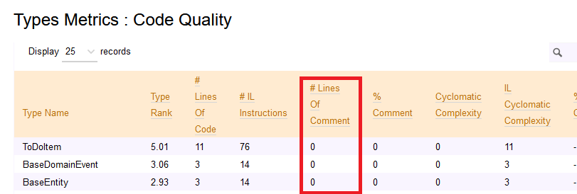
If you want to see the LOC value for your code, you can open the NDepend HTML report, head to Metrics > Types Metrics (in the left menu), and see that value.
This value is calculated based on the IL and the actual C# code, so it may happen that it’s not the exact number of lines you can see on your IDE. By the way, it’s a good estimation to understand which classes and methods need some attention.
Why is LOC important?
Keeping track of LOC is useful because the more lines of code, the more possible bugs.
Also, having lots of lines of code can make refactoring harder, especially because it’s probable that there is code duplication.
How to avoid it? Well, probably, you can’t. Or, at least, you can’t move to a lower magnitude. But, still, you can organize the code in modules with a small LOC value.
In this way, every LOC is easily maintainable, especially if focused on a specific aspect (SRP, anyone?)
The total LOC value won’t change. What will change is how the code is distributed across separated and independent modules.
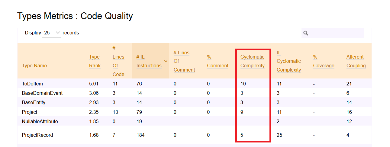
Cyclomatic complexity (CC)
Cyclomatic complexity is the measure of the number of linear paths through a module.
This formula works for simple programs and methods:
CC = E-N+2
where E is the number of Edges of the graph, while N is the number of Nodes.
Wait! Graph?? 😱
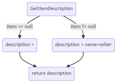
Code can be represented as a graph, where each node is a block of code.
Again, you will not calculate CC manually: we can use NDepend instead.
Calculating Cyclomatic Complexity with NDepend
As described before, the first step to do is to run NDepend and generate the HTML report. Then, open the left menu and click on Metrics > Type Metrics
Here you can see the values for Cyclomatic Complexity for every class (but you cannot drill down to every method).
Why is CC important?
Keeping track of Cyclomatic Complexity is good to understand the degree of complexity of a module or a method.
The higher the CC, the harder it will be to maintain and update the module.
We can use Cyclomatic Complexity as a lower limit for test cases. Since the CC of a method tells us about the number of independent execution paths, we can use that value to see the minimum number of tests to execute on that method. So, in the previous example, CC=2, and we need at least two tests: one for the case when item is null, and one for the case when item is not null.
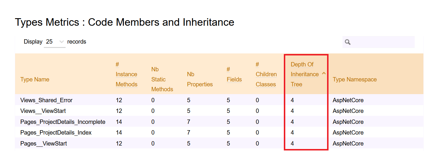
Depth of Inheritance Tree (DIT)
Depth of Inheritance Tree (DIT) is the value of the maximum length of the path between a base class and its farther subclass.
Take for example this simple class hierarchy.
publicclassUser{}
publicclassTeacher : User { }
publicclassStudent : User { }
publicclassAssociatedTeacher : Teacher { }
It can be represented as a tree, to better understand the relationship between classes:
Since the maximum depth of the tree is 3, the DIT value is 3.
How to calculate DIT with NDepend
As usual, run the code analysis with NDepend to generate the HTML report.
Then, you can head to Metrics > Type Metrics and navigate to the Code Members and Inheritance section to see the value of DIT of each class.
Why is DIT important?
Inheritance is a good way to reduce code duplication, that’s true: everything that is defined in the base class can be used by the derived classes.
But still, you should keep your eyes on the DIT value: if the depth level is greater than a certain amount (5, as stated by many devs), you’re probably risking to incur on possible bugs and unwanted behaviors due to some parent classes.
Also, having such a deep hierarchy may cause your system to be hard to maintain and evolve. So, if possible, prefer composition over inheritance.
Two words about NDepend
For sure, NDepend is an amazing tool for static analysis. All those metrics can be really useful – if you know how to use them. Luckily, not only do they give you the values of those metrics, but they also explain them.
In this article, I showed the most boring stuff you can see with NDepend. But you can do lots of incredible things.
My favorites ones are:
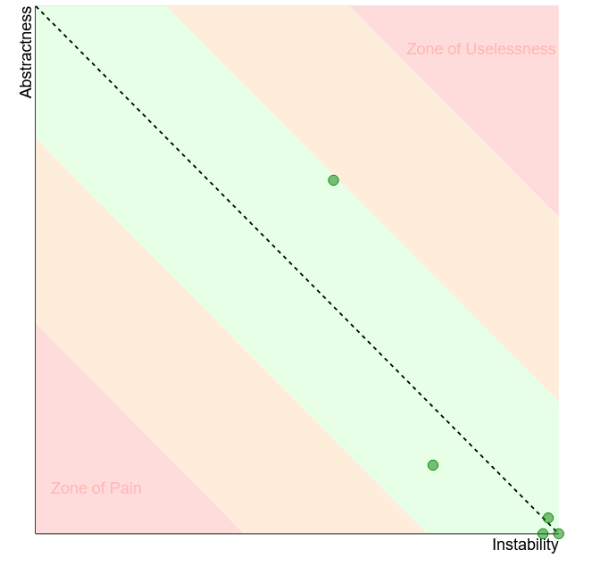
Instability vs Abstractness diagram, which shows if your modules are easy to maintain. The relation between Instability and Abstractness is well explained in Uncle Bob’s Clean Architecture book.
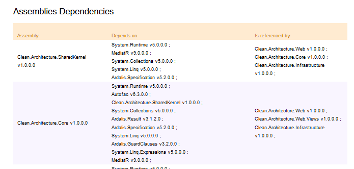
Assemblies Dependencies, which lists all the assemblies referenced by your project. Particularly useful to keep track of the OSS libraries you’re using, in case you need to update them for whichever reason (Log4J, anyone?)
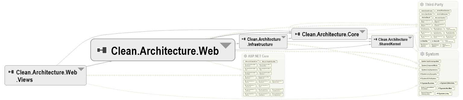
Then, the Component Dependencies Diagram, which is probably my fav feature: it allows you to navigate the modules and classes, and to understand which module depends on which other module.
and many more.
BUT!
There are also things I don’t like.
I found it difficult to get started with it: installing and running it the first time was quite difficult. Even updating it is not that smooth.
Then, the navigation menu is not that easy to understand. Take this screenshot:
Where can I find the Component Dependencies Diagram? Nowhere – it is accessible only from the homepage.
So, the tool is incredibly useful, but it’s difficult to use (at first, obviously).
If the NDepend team starts focusing on the usability and the UI, I’m sure it can quickly become a must-have tool for every team working on .NET. Of course, if they create a free (or cheaper) tier for their product with reduced capabilities: now it’s quite expensive. Well, actually it is quite cheap for companies, but for solo devs it is not affordable.
Additional resources
If you want to read more about how NDepend calculates those metrics, the best thing to do is to head to their documentation.
As I said before, you should avoid creating too many subclasses. Rather, you should compose objects to extend their behavior. A good way to do that is through the Decorator pattern, as I explained here.
In this article, we’ve seen how to measure metrics like Lines Of Code, Cyclomatic Complexity, and Depth of Inheritance Tree to keep an eye on the maintainability of a .NET solution.
To do that, we’ve used NDepend – I know, it’s WAY too powerful to be used only for those metrics. It’s like using a bazooka to kill a bee 🐝. But still, it was nice to try it out with a realistic project.
So, NDepend is incredibly useful for managing complex projects – it’s quite expensive, but in the long run, it may help you save money.
One of the best ways to learn is by recreating an interaction you’ve seen out in the wild and building it from scratch. It pushes you to notice the small details, understand the logic behind the animation, and strengthen your problem-solving skills along the way.
So today we’ll dive into rebuilding the smooth, draggable product grid from the Palmer website, originally crafted by Uncommon with Kevin Masselink, Alexis Sejourné, and Dylan Brouwer. The goal is to understand how this kind of interaction works under the hood and code the basics from scratch.
Along the way, you’ll learn how to structure a flexible grid, implement draggable navigation, and add smooth scroll-based movement. We’ll also explore how to animate products as they enter or leave the viewport, and finish with a polished product detail transition using Flip and SplitText for dynamic text reveals.
Let’s get started!
Grid Setup
The Markup
Let’s not try to be original and, as always, start with the basics. Before we get into the animations, we need a clear structure to work with — something simple, predictable, and easy to build upon.
What we have here is a .container that fills the viewport, inside of which sits a .grid divided into vertical columns. Each column stacks multiple .product elements, and every product wraps around an image. It’s a minimal setup, but it lays the foundation for the draggable, animated experience we’re about to create.
The Style
Now that we’ve got the structure, let’s add some styling to make the grid usable. We’ll keep things straightforward and use Flexbox instead of CSS Grid, since Flexbox makes it easier to handle vertical offsets for alternating columns. This approach keeps the layout flexible and ready for animation.
Okay, setup’s out of the way — now let’s jump into the fun part.
When developing interactive experiences, it helps to break things down into smaller parts. That way, each piece can be handled step by step without feeling overwhelming.
First, the grid isn’t centered by default, so we’ll fix that with a small utility function. This makes sure the grid always sits neatly in the middle of the screen, no matter the viewport size.
In the original Palmer reference, the experience starts with products appearing one by one in a slightly random order. After that reveal, the whole grid smoothly zooms into place.
To keep things simple, we’ll start with both the container and the products scaled down to 0.5 and the products fully transparent. Then we animate them back to full size and opacity, adding a random stagger so the images pop in at slightly different times.
The result is a dynamic but lightweight introduction that sets the tone for the rest of the interaction.
When you click on a product, an overlay opens and displays the product’s details. During this transition, the product’s image animates smoothly from its position in the grid to its position inside the overlay.
We build a simple overlay with minimal structure and styling and add an empty <div> that will contain the product image.
To achieve this effect, we use GSAP’s Flip plugin. This plugin makes it easy to animate elements between two states by calculating the differences in position, size, scale, and other properties, then animating them seamlessly.
We capture the state of the product image, move it into the details thumbnail container, and then animate the transition from the captured state to its new position and size.
I hope you enjoyed following along and picked up some useful techniques. Of course, there’s always room for further refinement—like experimenting with different easing functions or timing—but the core ideas are all here.
With this approach, you now have a handy toolkit for building smooth, draggable product grids or even simple image galleries. It’s something you can adapt and reuse in your own projects, and a good reminder of how much can be achieved with GSAP and its plugins when used thoughtfully.
A huge thanks to Codrops and to Manoela for giving me the opportunity to share this first article here 🙏 I’m really looking forward to hearing your feedback and thoughts!
Mapping every SQL result to a data type can be a pain. To simplify our life, we can use an ORM like Dapper to automatically map the data.
Table of Contents
Just a second! 🫷 If you are here, it means that you are a software developer.
So, you know that storage, networking, and domain management have a cost .
If you want to support this blog, please ensure that you have disabled the adblocker for this site. I configured Google AdSense to show as few ADS as possible – I don’t want to bother you with lots of ads, but I still need to add some to pay for the resources for my site.
Thank you for your understanding. – Davide
In a previous article, we’ve seen how to perform simple CRUD operations on a Postgres database by using Npgsql, a library that allows you to write and perform queries to be executed specifically on a PostgreSQL database.
In this article, we will take a step further: we will perform the same operations using Dapper, one of the most popular ORM for .NET applications, and we will see how performing those operations becomes easier.
Introducing the project
For this article, I will reuse the project I used for the previous article.
This project performs CRUD (Create, Read, Update, Delete) operations on a Postgres database with a single table: Games. All those operations (plus a bunch of other additional ones) are executed by a class that implements this interface:
This allows me to define and use a new class without modifying too much the project: in fact, I simply have to replace the dependency in the Startup class to use the Dapper repository.
But first…
Dapper, a micro-ORM
In the introduction, I said that we will use Dapper, a popular ORM. Let me explain.
ORM stands for Object-relational mapping and is a technique that allows you to map data from one format to another. This technique simplifies developers’ lives since they don’t have to manually map everything that comes from the database to an object – the ORM takes care of this task.
Dapper is one of the most popular ORMs, created by the Stack Overflow team. Well, actually Dapper is a Micro-ORM: it performs only a subset of the operations commonly executed by other ORMs; for example, Dapper allows you to map query results to objects, but it does not automatically generate the queries.
To add Dapper to your .NET project, simply run this command:
dotnet add package Dapper
Or add the NuGet package via Visual Studio:
Dapper will take care of only a part of the operations; for instance, it cannot open a connection to your DB. That’s why you need to install Npgsql, just as we did in a previous article. We can say the whole Dapper library is a set of Extension Methods built on top of the native data access implementation – in the case of PostgreSQL, on to op Npgsql.
Now we have all the dependencies installed, so we can start writing our queries.
Open the connection
Once we have created the application, we must instantiate and open a connection against our database.
private NpgsqlConnection connection;

public DapperBoardGameRepository()
{
    connection = new NpgsqlConnection(CONNECTION_STRING);
    connection.Open();
}
We will use the connection object later when we will perform the queries.
CRUD operations
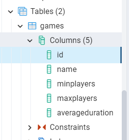
We are working on a table, Games, whose name is stored in a constant:
So, the main task of Dapper is to map the result of the queries performed on the Games table to one or more BoardGame objects.
Create
To create a new row on the Games table, we need to do something like this:
publicasync Task Add(BoardGame game)
{
string commandText = $"INSERT INTO {TABLE_NAME} (id, Name, MinPlayers, MaxPlayers, AverageDuration) VALUES (@id, @name, @minPl, @maxPl, @avgDur)";
var queryArguments = new
{
    id = game.Id,
    name = game.Name,
    minPl = game.MinPlayers,
    maxPl = game.MaxPlayers,
    avgDur = game.AverageDuration
};
await connection.ExecuteAsync(commandText, queryArguments);
}
Since Dapper does not create any queries for us, we still need to define them explicitly.
The query contains various parameters, marked with the @ symbol (@id, @name, @minPl, @maxPl, @avgDur). Those are placeholders, whose actual values are defined in the queryArguments anonymous object:
var queryArguments = new{
id = game.Id,
name = game.Name,
minPl = game.MinPlayers,
maxPl = game.MaxPlayers,
avgDur = game.AverageDuration
};
Finally, we can execute our query on the connection we have opened in the constructor:
When using Dapper, we declare the parameter values in a single anonymous object, and we don’t create a NpgsqlCommand instance to define our query.
Read
As we’ve seen before, an ORM simplifies how you read data from a database by automatically mapping the query result to a list of objects.
When we want to get all the games stored on our table, we can do something like that:
publicasync Task<IEnumerable<BoardGame>> GetAll()
{
string commandText = $"SELECT * FROM {TABLE_NAME}";
var games = await connection.QueryAsync<BoardGame>(commandText);
return games;
}
Again, we define our query and allow Dapper to do the rest for us.
In particular, connection.QueryAsync<BoardGame> fetches all the data from the query and converts it to a collection of BoardGame objects, performing the mapping for us.
Of course, you can also query for BoardGames with a specific Id:
publicasync Task<BoardGame> Get(int id)
{
string commandText = $"SELECT * FROM {TABLE_NAME} WHERE ID = @id";
var queryArgs = new { Id = id };
var game = await connection.QueryFirstAsync<BoardGame>(commandText, queryArgs);
return game;
}
As we did before, you define the query with a placeholder @id, which will have the value defined in the queryArgs anonymous object.
To store the result in a C# object, we map only the first object returned by the query, by using QueryFirstAsync instead of QueryAsync.
Comparison with Npgsql
The power of Dapper is the ability to automatically map query results to C# object.
With the plain Npgsql library, we would have done:
awaitusing (NpgsqlDataReader reader = await cmd.ExecuteReaderAsync())
while (await reader.ReadAsync())
{
BoardGame game = ReadBoardGame(reader);
games.Add(game);
}
to perform the query and open a reader on the result set. Then we would have defined a custom mapper to convert the Reader to a BoardGame object.
privatestatic BoardGame ReadBoardGame(NpgsqlDataReader reader)
{
int? id = reader["id"] asint?;
string name = reader["name"] asstring;
short? minPlayers = reader["minplayers"] as Int16?;
short? maxPlayers = reader["maxplayers"] as Int16?;
short? averageDuration = reader["averageduration"] as Int16?;
BoardGame game = new BoardGame
{
Id = id.Value,
Name = name,
MinPlayers = minPlayers.Value,
MaxPlayers = maxPlayers.Value,
AverageDuration = averageDuration.Value
};
return game;
}
With Dapper, all of this is done in a single instruction:
var games = await connection.QueryAsync<BoardGame>(commandText);
Update and Delete
Update and Delete operations are quite similar: just a query, with a parameter, whose operation is executed in an asynchronous way.
I will add them here just for completeness:
publicasync Task Update(int id, BoardGame game)
{
var commandText = $@"UPDATE {TABLE_NAME}
SET Name = @name, MinPlayers = @minPl, MaxPlayers = @maxPl, AverageDuration = @avgDur
WHERE id = @id";
var queryArgs = new {
id = game.Id,
name = game.Name,
minPl = game.MinPlayers,
maxPl = game.MaxPlayers,
avgDur = game.AverageDuration
};
await connection.ExecuteAsync(commandText, queryArgs);
}
and
publicasync Task Delete(int id)
{
string commandText = $"DELETE FROM {TABLE_NAME} WHERE ID=(@p)";
var queryArguments = new { p = id };
await connection.ExecuteAsync(commandText, queryArguments);
}
Again: define the SQL operation, specify the placeholders, and execute the operation with ExecuteAsync.
Further readings
As always, the best way to get started with a new library is by reading the official documentation:
Dapper adds a layer above the data access. If you want to go a level below, to have full control over what’s going on, you should use the native PostgreSQL library, Npgsql, as I explained in a previous article.
How to get a Postgres instance running? You can use any cloud implementation, or you can download and run a PostgreSQL instance on your local machine using Docker as I explained in this guide:
In this article, we’ve seen how to use Dapper to simplify our data access. Dapper is useful for querying different types of RDBMS, not only PostgreSQL.
To try those examples out, download the code from GitHub, specify the connection string, and make sure that you are using the DapperBoardGameRepository class (this can be configured in the Startup class).
In a future article, we will use Entity Framework to – guess what? – perform CRUD operations on the Games table. In that way, you will have 3 different ways to access data stored on PostgreSQL by using .NET Core.
With Entity Framework you can perform operations on relational databases without writing a single line of SQL. We will use EF to integrate PostgreSQL in our application
Table of Contents
Just a second! 🫷 If you are here, it means that you are a software developer.
So, you know that storage, networking, and domain management have a cost .
If you want to support this blog, please ensure that you have disabled the adblocker for this site. I configured Google AdSense to show as few ADS as possible – I don’t want to bother you with lots of ads, but I still need to add some to pay for the resources for my site.
Thank you for your understanding. – Davide
When working with relational databases, you often come across two tasks: writing SQL queries and mapping the results to some DTO objects.
.NET developers are lucky to have an incredibly powerful tool that can speed up their development: Entity Framework. Entity Framework (in short: EF) is an ORM built with in mind simplicity and readability.
In this article, we will perform CRUD operations with Entity Framework Core on a database table stored on PostgreSQL.
Introduction EF Core
With Entity Framework you don’t have to write SQL queries in plain text: you write C# code that gets automatically translated into SQL commands. Then the result is automatically mapped to your C# classes.
Entity Framework supports tons of database engines, such as SQL Server, MySQL, Azure CosmosDB, Oracle, and, of course, PostgreSQL.
There are a lot of things you should know about EF if you’re new to it. In this case, the best resource is its official documentation.
But the only way to learn it is by getting your hands dirty. Let’s go!
How to set up EF Core
For this article, we will reuse the same .NET Core repository and the same database table we used when we performed CRUD operations with Dapper (a lightweight OR-M) and with NpgSql, which is the library that performs bare-metal operations.
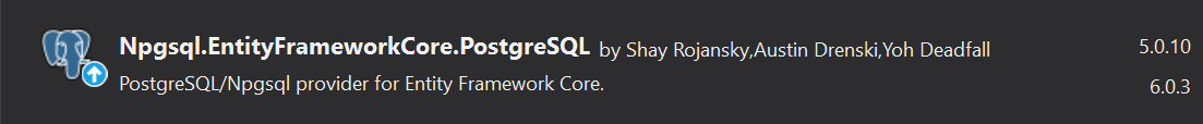
The first thing to do is, as usual, install the related NuGet package. Here we will need Npgsql.EntityFrameworkCore.PostgreSQL. Since I’ve used .NET 5, I have downloaded version 5.0.10.
Then, we need to define and configure the DB Context.
Define and configure DbContext
The idea behind Entity Framework is to create DB Context objects that map database tables to C# data sets. DB Contexts are the entry point to the tables, and the EF way to work with databases.
So, the first thing to do is to define a class that inherits from DbContext:
publicclassBoardGamesContext : DbContext
{
}
Within this class we define one or more DbSets, that represent the collections of data rows on their related DB table:
public DbSet<BoardGame> Games { get; set; }
Then we can configure this specific DbContext by overriding the OnConfiguring method and specifying some options; for example, you can specify the connection string:
Now that we have the BoardGamesContext ready we have to add its reference in the Startup class.
In the ConfigureServices method, add the following instruction:
services.AddDbContext<BoardGamesContext>();
With this instruction, you make the BoardGamesContext context available across the whole application.
You can further configure that context using an additional parameter of type Action<DbContextOptionsBuilder>. In this example, you can skip it, since we’ve already configured the BoardGamesContext using the OnConfiguring method. They are equivalent.
As we know, EF allows you to map DB rows to C# objects. So, we have to create a class and configure it in a way that allows EF Core to perform the mapping.
Now that the setup is complete, we can perform our CRUD operations. Entity Framework simplifies a lot the way to perform such types of operations, so we can move fast in this part.
There are two main points to remember:
to access the context we have to create a new instance of BoardGamesContext, which should be placed into a using block.
When performing operations that change the status of the DB (insert/update/delete rows), you have to explicitly call SaveChanges or SaveChangesAsync to apply those changes. This is useful when performing batch operations on one or more tables (for example, inserting an order in the Order table and updating the user address in the Users table).
Create
To add a new BoardGame, we have to initialize the BoardGamesContext context and add a new game to the Games DbSet.
publicasync Task Add(BoardGame game)
{
using (var db = new BoardGamesContext())
{
await db.Games.AddAsync(game);
await db.SaveChangesAsync();
}
}
Read
If you need a specific entity by its id you can use Find and FindAsync.
publicasync Task<BoardGame> Get(int id)
{
using (var db = new BoardGamesContext())
{
returnawait db.Games.FindAsync(id);
}
}
Or, if you need all the items, you can retrieve them by using ToListAsync
publicasync Task<IEnumerable<BoardGame>> GetAll()
{
using (var db = new BoardGamesContext())
{
returnawait db.Games.ToListAsync();
}
}
Update
Updating an item is incredibly straightforward: you have to call the Update method, and then save your changes with SaveChangesAsync.
publicasync Task Update(int id, BoardGame game)
{
using (var db = new BoardGamesContext())
{
db.Games.Update(game);
await db.SaveChangesAsync();
}
}
For some reason, EF does not provide an asynchronous way to update and remove items. I suppose that it’s done to prevent or mitigate race conditions.
Delete
Finally, to delete an item you have to call the Remove method and pass to it the game to be removed. Of course, you can retrieve that game using FindAsync.
publicasync Task Delete(int id)
{
using (var db = new BoardGamesContext())
{
var game = await db.Games.FindAsync(id);
if (game == null)
return;
db.Games.Remove(game);
await db.SaveChangesAsync();
}
}
Further readings
Entity Framework is impressive, and you can integrate it with tons of database vendors. In the link below you can find the full list. But pay attention that not all the libraries are implemented by the EF team, some are third-party libraries (like the one we used for Postgres):
This article concludes the series that explores 3 ways to perform CRUD operations on a Postgres database with C#.
In the first article, we’ve seen how to perform bare-metal queries using NpgSql. In the second article, we’ve used Dapper, which helps mapping queries results to C# DTOs. Finally, we’ve used Entity Framework to avoid writing SQL queries and have everything in place.
Which one is your favorite way to query relational databases?
SeedTodos – quickly inserts a few sample todos into the API, so we don’t start from an empty sheet.
ListTodosToSheet – pulls all todos into Sheet1. It writes ID, Title, and Completed columns, so you can see the live state.
DumpTodosToImmediate – prints the same list into the VBA Immediate Window (Ctrl+G). Handy for quick debugging.
?CreateTodo(“Watch VitoshAcademy”,True) – creates a new todo with a title and completed flag. The ? in the Immediate Window prints the returned ID.
UpdateTodoTitle1,“Watch VitoshAcademy” – updates the title of the todo with ID=1.
SetTodoCompleted1,True – marks the same item as completed.
GetTodoById1 – fetches a single item as raw JSON, displayed in the Immediate Window.
DeleteTodo1 – removes the todo with ID=1.
DeleteAllTodos – wipes everything in the list (careful with this one!).
ListTodosToSheet – refresh the sheet after changes to confirm results.
PushSheetToApi – the powerful one: reads rows from Excel (ID, Title, Completed, Action) and syncs them back to the API. That way you can create, update, or delete tasks directly from the sheet.
With these simple commands, Excel is no longer just a spreadsheet — it’s a lightweight API client. And because the backend runs in Docker, the setup is reproducible and isolated. This small project connects three different worlds — Docker, Python, and Excel VBA. It is a demonstration that APIs are not only for web developers; even Excel can talk to them easily.
After 100 articles, I’ve found some neat ways to automate my blogging workflow. I will share my experience and the tools I use from the very beginning to the very end.
Table of Contents
Just a second! 🫷 If you are here, it means that you are a software developer.
So, you know that storage, networking, and domain management have a cost .
If you want to support this blog, please ensure that you have disabled the adblocker for this site. I configured Google AdSense to show as few ADS as possible – I don’t want to bother you with lots of ads, but I still need to add some to pay for the resources for my site.
Thank you for your understanding. – Davide
This is my 100th article 🥳 To celebrate it, I want to share with you the full process I use for writing and publishing articles.
In this article I will share all the automation and tools I use for writing, starting from the moment an idea for an article pops up in my mind to what happens weeks after an article has been published.
I hope to give you some ideas to speed up your publishing process. Of course, I’m open to suggestions to improve my own flow: perhaps (well, certainly), you use better tools and processes, so feel free to share them.
Introducing my blog architecture
To better understand what’s going on, I need a very brief overview of the architecture of my blog.
It is written in Gatsby, a framework based on ReactJS that, in short, allows you to transform Markdown files into blog posts (it does many other things, but they are not important for the purpose of this article).
So, all my blog is stored in a private GitHub repository. Every time I push some changes on the master branch, a new deployment is triggered, and I can see my changes in a bunch of minutes on my blog.
As I said, I use Gatsby. But the key point here is that my blog is stored in a GitHub repo: this means that everything you’ll read here is valid for any Headless CMS based on Git, such as Gatsby, Hugo, NextJS, and Jekyll.
Now that you know some general aspects, it’s time to deep dive into my writing process.
Before writing: organizing ideas with GitHub
My central source, as you might have already understood, is GitHub.
There, I write all my notes and keep track of the status of my articles.
Everything is quite well organized, and with the support of some automation, I can speed up my publishing process.
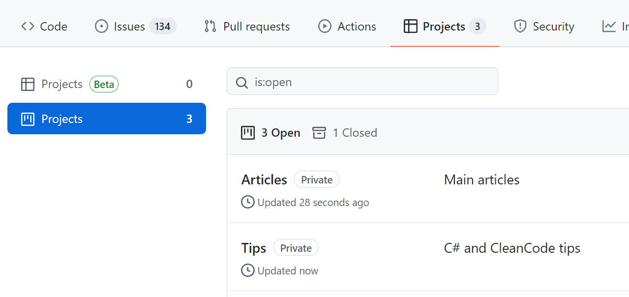
Github Projects to track the status of the articles
GitHub Projects are the parts of GitHub that allow you to organize GitHub Issues to track their status.
I’ve created 2 GitHub Projects: one for the main articles (like this one), and one for my C# and Clean Code Tips.
In this way, I can use different columns and have more flexibility when handling the status of the tasks.
GitHub issues templates
As I said, to write my notes I use GitHub issues.
When I add a new Issue, the first thing is to define which type of article I want to write. And, since sometimes many weeks or months pass between when I came up with the idea for an article and when I start writing it, I need to organize my ideas in a structured way.
To do that, I use GitHub templates. When I create a new Issue, I choose which kind of article I’m going to write.
Based on the layout, I can add different info. For instance, when I want to write a new “main” article, I see this form
which is prepopulated with some fields:
Title: with a placeholder ([Article] )
Content: with some sections (the titles, translated from Italian, mean Topics, Links, General notes)
Labels: I automatically assign the Article label to the issue (you’ll see later why I do that)
How can you create GitHub issue templates? All you need is a Markdown file under the .github/ISSUE_TEMPLATE folder with content similar to this one.
---
name: New article
about: New blog article
title: "[Article] - "
labels: Article
assignees: bellons91
---

## Argomenti

## Link

## Appunti vari
And you’re good to go!
GitHub action to assign issues to a project
Now I have GitHub Projects and different GitHub Issues Templates. How can I join the different parts? Well, with GitHub Actions!
With GitHub Actions, you can automate almost everything that happens in GitHub (and outside) using YAML files.
So, here’s mine:
For better readability, you can find the Gist here.
This action looks for opened and labeled issues and pull requests, and based on the value of the label it assigns the element to the correct project.
In this way, after I choose a template, filled the fields, and added additional labels (like C#, Docker, and so on), I can see my newly created issue directly in the Articles board. Neat 😎
Writing
Now it’s the time of writing!
As I said, I’m using Gatsby, so all my articles are stored in a GitHub repository and written in Markdown.
For every article I write, I use a separate git branch: in this way, I’m free to update the content already online (in case of a typo) without publishing my drafts.
But, of course, I automated it! 😎
Powershell script to scaffold a new article
Every article lives in its /content/posts/{year}/{folder-name}/article.md file. And they all have a cover image in a file named cover.png.
Also, every MD file begins with a Frontmatter section, like this:
---
title: "How I automated my publishing flow with Gatsby, GitHub, PowerShell and Azure"
path: "/blog/automate-articles-creations-github-powershell-azure"
tags: ["MainArticle"]
featuredImage: "./cover.png"
excerpt: "a description for 072-how-i-create-articles"
created: 4219-11-20
updated: 4219-11-20
---
But, you know, I was tired of creating everything from scratch. So I wrote a Powershell Script to do everything for me.
where article-creator.ps1 is the name of the file that contains the script.
Now I can simply run npm run create-article to have a new empty article in a new branch, already updated with everything published in the Master branch.
Markdown preview on VS Code
I use Visual Studio Code to write my articles: I like it because it’s quite fast and with lots of functionalities to write in Markdown (you can pick your favorites in the Extensions store).
One of my favorites is the Preview on Side. To see the result of your MarkDown on a side panel, press CTRL+SHIFT+P and select Open Preview to the Side.
Here’s what I can see right now while I’m writing:
Grammar check with Grammarly
Then, it’s time for a check on the Grammar. I use Grammarly, which helps me fix lots of errors (well, in the last time, only a few: it means I’ve improved a lot! 😎).
I copy the Markdown in their online editor, fix the issues, and copy it back into my repo.
Fun fact: the online editor recognizes that you’re using Markdown and automatically checks only the actual text, ignoring all the symbols you use in Markdown (like brackets).
Unprofessional, but fun, cover images
One of the tasks I like the most is creating my cover images.
I don’t use stock images, I prefer using less professional but more original cover images.
Creating and scheduling PR on GitHub with Templates and Actions
Now that my article is complete, I can set it as ready for being scheduled.
To do that, I open a Pull Request to the Master Branch, and, again, add some kind of automation!
I have created a PR template in an MD file, which I use to create a draft of the PR content.
In this way, I can define which task (so, which article) is related to this PR, using the “Closes” formula (“Closes #111174” means that I’m closing the Issue with ID 111174).
Also, I can define when this PR will be merged on Master, using the /schedule tag.
It works because I have integrated into my workflow a GitHub Action, merge-schedule, that reads the date from that field to understand when the PR must be merged.
So, every Tuesday at 8 AM, this action runs to check if there are any PRs that can be merged. If so, the PR will be merged into master, and the CI/CD pipeline builds the site and publishes the new content.
As usual, you can find the code of this action here
After the PR is merged, I also receive an email that notifies me of the action.
After publishing
Once a new article is online, I like to give it some visibility.
To do that, I heavily rely on Azure Logic Apps.
Azure Logic App for sharing on Twitter
My blog exposes an RSS feed. And, obviously, when a new article is created, a new item appears in the feed.
I use it to trigger an Azure Logic App to publish a message on Twitter:
The Logic App reads the newly published feed item and uses its metadata to create a message that will be shared on Twitter.
If you prefer, you can use a custom Azure Function! The choice is yours!
Cross-post reminder with Azure Logic Apps
Similarly, I use an Azure Logic App to send to myself an email to remind me to cross-post my articles to other platforms.
I’ve added a delay so that my content lives longer, and I can repost it even after weeks or months.
Unluckily, when I cross-post my articles I have to do it manually, This is quite a time-consuming especially when there are lots of images: in my MD files I use relative paths, so when porting my content to different platforms I have to find the absolute URL for my images.
And, my friends, this is everything that happens in the background of my blog!
What I’m still missing
I’ve added a lot of effort to my blog, and I’m incredibly proud of it!
But still, there are a few things I’d like to improve.
SEO Tools/analysis
I’ve never considered SEO. Or, better, Keywords.
I write for the sake of writing, and because I love it. And I don’t like to stuff my content with keywords just to rank better on search engines.
I take care of everything like alt texts, well-structured sections, and everything else. But I’m not able to follow the “rules” to find the best keywords.
Maybe I should use some SEO tools to find the best keywords for me. But I don’t want to bend to that way of creating content.
Also, I should spend more time thinking of the correct title and section titles.
Any idea?
Easy upgrade of Gatsby/Migrate to other headless CMSs
Lastly, I’d like to find another theme or platform and leave the one I’m currently using.
Not because I don’t like it. But because many dependencies are outdated, and the theme I’m using hasn’t been updated since 2019.
Wrapping up
That’s it: in this article, I’ve explained everything that I do when writing a blog post.
Feel free to take inspiration from my automation to improve your own workflow, and contact me if you have some nice improvements or ideas: I’m all ears!
In today’s regulatory climate, compliance is no longer a box-ticking exercise. It is a strategic necessity. Organizations across industries are under pressure to secure sensitive data, meet privacy obligations, and avoid hefty penalties. Yet, despite all the talk about “data visibility” and “compliance readiness,” one fundamental gap remains: unseen data—the information your business holds but doesn’t know about.
Unseen data isn’t just a blind spot—it’s a compliance time bomb waiting to trigger regulatory and reputational damage.
The Myth: Sensitive Data Lives Only in Databases
Many businesses operate under the dangerous assumption that sensitive information exists only in structured repositories like databases, ERP platforms, or CRM systems. While it’s true these systems hold vast amounts of personal and financial information, they’re far from the whole picture.
Reality check: Sensitive data is often scattered across endpoints, collaboration platforms, and forgotten storage locations. Think of HR documents on a laptop, customer details in a shared folder, or financial reports in someone’s email archive. These are prime targets for breaches—and they often escape compliance audits because they live outside the “official” data sources.
Myth vs Reality: Why Structured Data is Not the Whole Story
Yes, structured sources like SQL databases allow centralized access control and auditing. But compliance risks aren’t limited to structured data. Unstructured and endpoint data can be far more dangerous because:
They are harder to track.
They often bypass IT policies.
They get replicated in multiple places without oversight.
When organizations focus solely on structured data, they risk overlooking up to 50–70% of their sensitive information footprint.
The Challenge Without Complete Discovery
Without full-spectrum data discovery—covering structured, unstructured, and endpoint environments—organizations face several challenges:
Compliance Gaps – Regulations like GDPR, DPDPA, HIPAA, and CCPA require knowing all locations of personal data. If data is missed, compliance reports will be incomplete.
Increased Breach Risk – Cybercriminals exploit the easiest entry points, often targeting endpoints and poorly secured file shares.
Inefficient Remediation – Without knowing where data lives, security teams can’t effectively remove, encrypt, or mask it.
Costly Investigations – Post-breach forensics becomes slower and more expensive when data locations are unknown.
The Importance of Discovering Data Everywhere
A truly compliant organization knows where every piece of sensitive data resides, no matter the format or location. That means extending discovery capabilities to:
Structured Data
Where it lives: Databases, ERP, CRM, and transactional systems.
Why it matters: It holds core business-critical records, such as customer PII, payment data, and medical records.
Risks if ignored: Non-compliance with data subject rights requests; inaccurate reporting.
Unstructured Data
Where it lives: File servers, SharePoint, Teams, Slack, email archives, cloud storage.
Why it matters: Contains contracts, scanned IDs, reports, and sensitive documents in freeform formats.
Risks if ignored: Harder to monitor, control, and protect due to scattered storage.
Endpoint Data
Where it lives: Laptops, desktops, mobile devices (Windows, Mac, Linux).
Why it matters: Employees often store working copies of sensitive files locally.
Risks if ignored: Theft, loss, or compromise of devices can expose critical information.
Real-World Examples of Compliance Risks from Unseen Data
Healthcare Sector: A hospital’s breach investigation revealed patient records stored on a doctor’s laptop, which was never logged into official systems. GDPR fines followed.
Banking & Finance: An audit found loan application forms with customer PII on a shared drive, accessible to interns.
Retail: During a PCI DSS assessment, old CSV exports containing cardholder data were discovered in an unused cloud folder.
Government: Sensitive citizen records are emailed between departments, bypassing secure document transfer systems, and are later exposed to a phishing attack.
Closing the Gap: A Proactive Approach to Data Discovery
The only way to eliminate unseen data risks is to deploy comprehensive data discovery and classification tools that scan across servers, cloud platforms, and endpoints—automatically detecting sensitive content wherever it resides.
This proactive approach supports regulatory compliance, improves breach resilience, reduces audit stress, and ensures that data governance policies are meaningful in practice, not just on paper.
Bottom Line
Compliance isn’t just about protecting data you know exists—it’s about uncovering the data you don’t. From servers to endpoints, organizations need end-to-end visibility to safeguard against unseen risks and meet today’s stringent data protection laws.